Author Bernhard AhrensAuthor Lazaro Alonso

---

Hyperparameter tuning with Hyperopt.jl

1. Setup and Data Loading

Load package and synthetic dataset

using EasyHybrid
using CairoMakie
using Hyperopt

ds = load_timeseries_netcdf("https://github.com/bask0/q10hybrid/raw/master/data/Synthetic4BookChap.nc")
ds = ds[1:20000, :]  # Use subset for faster execution
first(ds, 5)

5×6 DataFrame

Row	time	sw_pot	dsw_pot	ta	reco	rb
	DateTime	Float64?	Float64?	Float64?	Float64?	Float64?
1	2003-01-01T00:15:00	109.817	115.595	2.1	0.844741	1.42522
2	2003-01-01T00:45:00	109.817	115.595	1.98	0.840641	1.42522
3	2003-01-01T01:15:00	109.817	115.595	1.89	0.837579	1.42522
4	2003-01-01T01:45:00	109.817	115.595	2.06	0.843372	1.42522
5	2003-01-01T02:15:00	109.817	115.595	2.09	0.844399	1.42522

2. Define the Process-based Model

RbQ10 model: Respiration model with Q10 temperature sensitivity

function RbQ10(;ta, Q10, rb, tref = 15.0f0)
    reco = rb .* Q10 .^ (0.1f0 .* (ta .- tref))
    return (; reco, Q10, rb)
end

RbQ10 (generic function with 1 method)

3. Configure Model Parameters

Parameter specification: (default, lower_bound, upper_bound)

parameters = (
    rb  = (3.0f0, 0.0f0, 13.0f0),  # Basal respiration [μmol/m²/s]
    Q10 = (2.0f0, 1.0f0, 4.0f0),   # Temperature sensitivity - describes factor by which respiration is increased for 10 K increase in temperature [-]
)

(rb = (3.0f0, 0.0f0, 13.0f0), Q10 = (2.0f0, 1.0f0, 4.0f0))

4. Construct the Hybrid Model

Define input variables

forcing = [:ta]                    # Forcing variables (temperature)
predictors = [:sw_pot, :dsw_pot]   # Predictor variables (solar radiation)
target = [:reco]                   # Target variable (respiration)

1-element Vector{Symbol}:
 :reco

Parameter classification as global, neural or fixed (difference between global and neural)

global_param_names = [:Q10]        # Global parameters (same for all samples)
neural_param_names = [:rb]         # Neural network predicted parameters

1-element Vector{Symbol}:
 :rb

Construct hybrid model

hybrid_model = constructHybridModel(
    predictors,               # Input features
    forcing,                  # Forcing variables
    target,                   # Target variables
    RbQ10,                    # Process-based model function
    parameters,               # Parameter definitions
    neural_param_names,       # NN-predicted parameters
    global_param_names,       # Global parameters
    hidden_layers = [16, 16], # Neural network architecture
    activation = relu,       # Activation function
    scale_nn_outputs = true,  # Scale neural network outputs
    input_batchnorm = false    # Apply batch normalization to inputs
)

Hybrid Model (Single NN)
Neural Network: 
  Chain(
      layer_1 = WrappedFunction(identity),
      layer_2 = Dense(2 => 16, relu),               # 48 parameters
      layer_3 = Dense(16 => 16, relu),              # 272 parameters
      layer_4 = Dense(16 => 1),                     # 17 parameters
  )         # Total: 337 parameters,
            #        plus 0 states.
Configuration:
  mechanistic_model = RbQ10
  targets = [:reco]
  forcing = [:ta]
  neural_param_names = [:rb]
  predictors = [:sw_pot, :dsw_pot]
  global_param_names = [:Q10]
  fixed_param_names = Symbol[]
  scale_nn_outputs = true
  start_from_default = true
  config = (; hidden_layers = [16, 16], activation = relu, scale_nn_outputs = true, input_batchnorm = false, start_from_default = true,)

Parameters:
  ┌─────┬────────┬───────┬───────┬────────┐
  │     │  value │ lower │ upper │  scale │
  ├─────┼────────┼───────┼───────┼────────┤
  │  rb │     NN │   0.0 │  13.0 │ linear │
  │ Q10 │ Global │   1.0 │   4.0 │ linear │
  └─────┴────────┴───────┴───────┴────────┘
  value: number = fixed; NN/Global = estimated; Forcing = overridden by forcing data

5. Train the Model

out = train(
    hybrid_model,
    ds,
    ();
    nepochs = 100,               # Number of training epochs
    batchsize = 512,             # Batch size for training
    opt = AdamW(0.001),        # Optimizer and learning rate
    monitor_names = [:rb, :Q10], # Parameters to monitor during training
    yscale = identity,           # Scaling for outputs
    patience = 30,               # Early stopping patience
    show_progress=false,
    hybrid_name="before"
)

  train_history: (31,)
    mse  (reco, sum)
    r2   (reco, sum)
  val_history: (31,)
    mse  (reco, sum)
    r2   (reco, sum)
  epoch_history: (31,)
    l_train  (mse, r2)
    l_val    (mse, r2)
    ŷ_train  (reco, Q10, rb, parameters)
    ŷ_val    (reco, Q10, rb, parameters)
  train_obs_pred: 16000×2 DataFrame
    reco, reco_pred
  val_obs_pred: 4000×2 DataFrame
    reco, reco_pred
  train_diffs: 
    Q10         (1,)
    rb          (16000,)
    parameters  (rb, Q10)
  val_diffs: 
    Q10         (1,)
    rb          (4000,)
    parameters  (rb, Q10)
  ps: 
    ps   (layer_1, layer_2, layer_3, layer_4)
    Q10  (1,)
  st: 
    st_nn  (layer_1, layer_2, layer_3, layer_4)
    fixed  ()
  best_epoch: 0
  best_loss: 14.315285

6. Check Results

Evolution of train and validation loss

EasyHybrid.plot_loss(out, yscale = identity)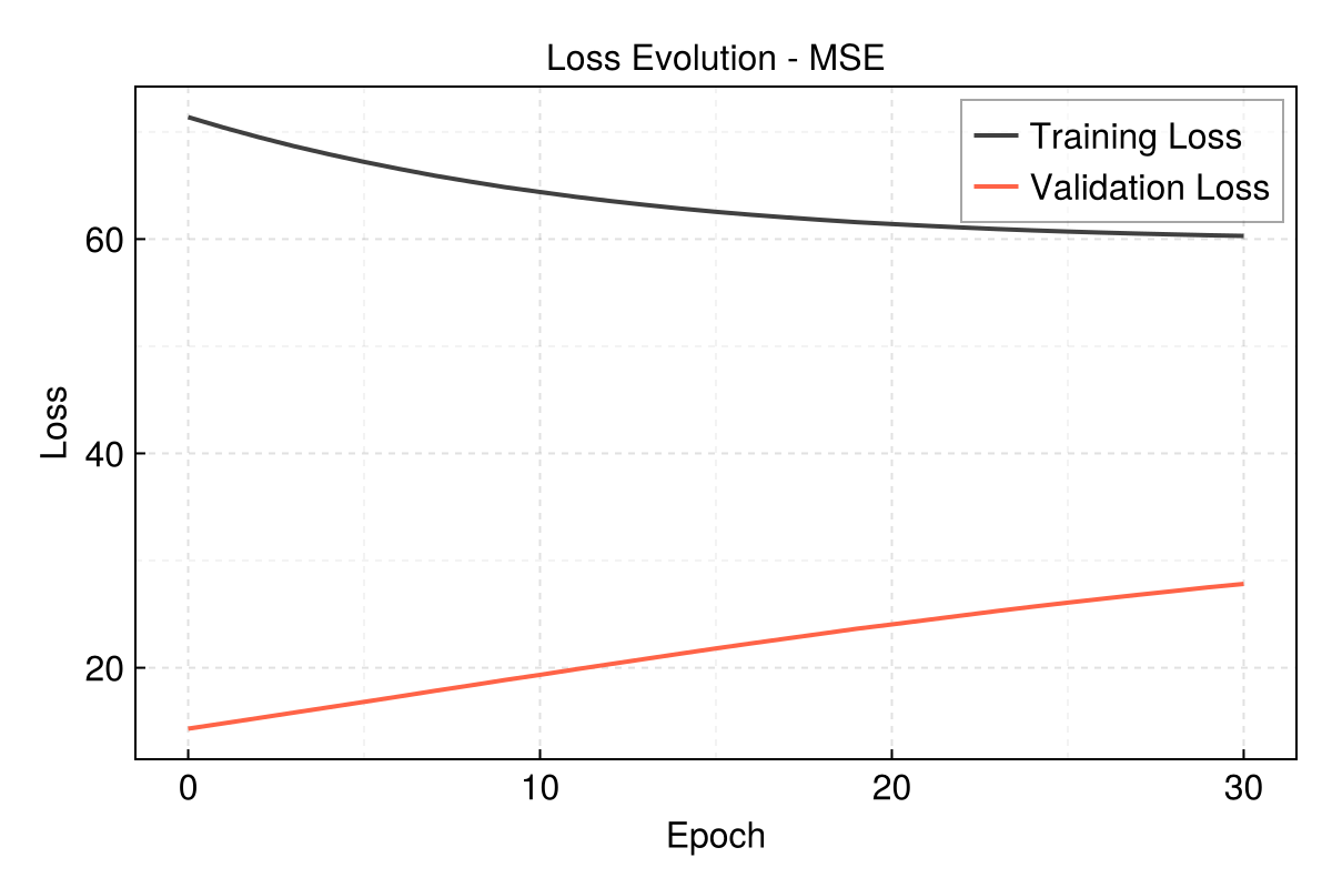

Check results - what do you think - is it the true Q10 used to generate the synthetic dataset?

out.train_diffs.Q10

1-element Vector{Float32}:
 2.0

Quick scatterplot - dispatches on the output of train

EasyHybrid.poplot(out)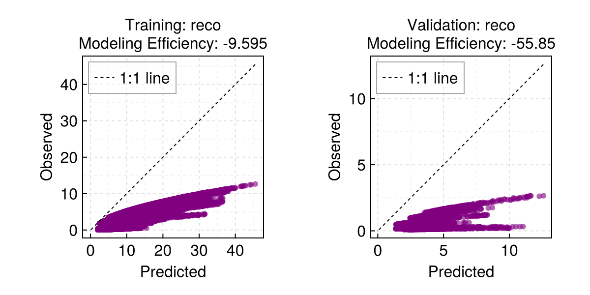

Hyperparameter Tuning

EasyHybrid provides built-in hyperparameter tuning capabilities to optimize your model configuration. This is especially useful for finding the best neural network architecture, optimizer settings, and other hyperparameters.

Basic Hyperparameter Tuning

You can use the tune function to automatically search for optimal hyperparameters. Check Hyperopt.jl for details on algorithms.

# Create empty model specification for tuning
mspempty = ModelSpec()

# Define hyperparameter search space
nhyper = 4
# For actual parallel runs, change `@hyperopt` to `@thyperopt` below.
ho = @hyperopt for i=nhyper,
    opt = [AdamW(0.01), AdamW(0.1), RMSProp(0.001), RMSProp(0.01)],
    input_batchnorm = [true, false]

    hyper_parameters = (;opt, input_batchnorm)
    println("Hyperparameter run: ", i, " of ", nhyper, " with hyperparameters: ", hyper_parameters)

    # Run tuning with current hyperparameters
    out = EasyHybrid.tune(
        hybrid_model,
        ds,
        mspempty;
        hyper_parameters...,
        nepochs = 10,
        plotting = false,
        show_progress = false,
        file_name = "test$i.jld2",
        model_name = "model_$(i)"
    )

    out.best_loss
end

# Get the best hyperparameters
ho.minimizer
printmin(ho)

# Train the model with the best hyperparameters
best_hyperp = best_hyperparams(ho)

(opt = RMSProp(eta=0.001, rho=0.9, epsilon=1.0e-8, centred=false, input_batchnorm = true)

Train model with the best hyperparameters

# Run tuning with specific hyperparameters
out_tuned = EasyHybrid.tune(
    hybrid_model,
    ds,
    mspempty;
    best_hyperp...,
    nepochs = 100,
    monitor_names = [:rb, :Q10],
    hybrid_name="after"
)

# Check the tuned model performance
out_tuned.best_loss

0.0011609511f0

Key Hyperparameters to Tune

When tuning your hybrid model, consider these important hyperparameters:

• Optimizer and Learning Rate: Try different optimizers (AdamW, RMSProp, Adam) with various learning rates

• Neural Network Architecture: Experiment with different hidden_layers configurations

• Activation Functions: Test different activation functions (relu, sigmoid, tanh)

• Batch Normalization: Enable/disable input_batchnorm and other normalization options

• Batch Size: Adjust batchsize for optimal training performance

Tips for Hyperparameter Tuning

• Start with a small search space to get a baseline understanding

• Monitor for overfitting by tracking validation loss

• Consider computational cost - more hyperparameters and epochs increase training time

More Examples

Check out the overview page for additional examples and use cases. Each project demonstrates different aspects of hybrid modeling with EasyHybrid.