Makie Helpers

Unit conversions

Many graphical properties are given in pixel or inches. Working with figures for international journals, however, usually requires thinking and specification in metric units. The following function help to convert.

FigureHelpers.cm2inch — Function

cm2inch(x)
cm2inch(x1, x2, x...)

Convert length in cm to inch units: 1 inch = 2.54 The single argument returns a value, the multiple argument version a Tuple. Similar to more verbose syntax using Unitful.jl: uconvert(u"inch",x * u"cm").val.

source

Figures often look well, if the ratio between length and height corresponds to the Golden ratio. So we provide it here.

FigureHelpers.golden_ratio — Constant

golden_ratio ≈ 1.618

Two quantities are in the golden ratio if their ratio is the same as the ratio of their sum to the larger of the two quantities.

source

Makie Layout switching and Figure generation

Generating the same plot for paper and for a presentation, requires adjusting properties such as figure sizes, fontsizes, and graphics format. The following class helps to collect them and provide them to functions below

FigureHelpers.MakieConfig — Type

MakieConfig

A collection of figure properties to tailor the same figure either for presentation in a paper or a presentation.

Properties and defaults

pt_per_unit = 0.75
px_per_unit = 2.0
filetype = "svg"
fontsize = 9 (point units)
size_inches = cm2inch.((17.5,17.5/golden_ratio)) (width x height)

The default px_per_unit needs to rescale a png image in ppt to 50%, but this gives better quality.

source

FigureHelpers.paper_MakieConfig — Function

paper_MakieConfig(;
    target = :paper, filetype = "pdf", 
    fontsize=9, size_inches = cm2inch.((8.3,8.3/golden_ratio)), ...)    
    
ppt_MakieConfig(;
    target = :presentation, filetype = "svg", 
    fontsize=18, size_inches = (6.65,6.65/golden_ratio), ...)

png_MakieConfig(;target = :png, filetype = "png", ...)

Specialized configurations adapted to

paper_MakieConfig: single column Biogeosciences paper (8.3cm)
ppt_MakieConfig: half of a wide-screen ppt presentation (13.3 inch), either svg or png Inserting generated svg yields better quality than copy (=png) from VScode preview.
png_MakieConfig: same as ppt, but generating png images at 200% scale By default, need to rescale the png to 50% when inserting into presentation.

source

creating Makie Figures with adjusted sizes and font-sizes

FigureHelpers.figure_conf — Function

figure_conf(; makie_config)
figure_conf(width2height, xfac=1.0; makie_config)

figure_conf(size_inches = cm2inch.((8.3,8.3/golden_ratio)); fontsize=9, pt_per_unit = 0.75)

Creates a figure with specified resolution/size and fontsize for given figure size.

The first two constructors apply the settings from the config, with the possibility to adjust the width/height ration (e.g. to golden_ratio) or multiply the default x-width.

The last constructor sets the properties without referring to a config. It uses by default pt_per_unit=0.75 to conform to png display and save. Remember to divide fontsize and other sizes specified elsewhere by this factor. See also cm2inch and save.

source

FigureHelpers.figure_conf_axis — Function

figure_conf_axis(...; makie_config, kwrags...)

Call figure_conf but return a tuple (figure, axis). The keyword arguments are passed to the Axis(; kwrawgs...) call.

source

saving figures to correct format, subdirectory, and dpi-resolution

FigureHelpers.save_with_config — Function

save_with_config(filename, fig; makie_config = MakieConfig(), args...)

Save figure with file updated extension cfg.filetype to subdirectory cfg.filetype of given path of filename. Sets pt_per_unit and px_per_unit according to makie_config.

source

Shortcuts

FigureHelpers.hidexdecoration! — Function

hidexdecoration!(ax;, label, ticklabels, ticks, grid, minorgrid, minorticks; kwargs...)
hideydecoration!(ax;, label, ticklabels, ticks, grid, minorgrid, minorticks; kwargs...)

Versions of hidexdecorations! and hideydecorations! with defaults reversed. This allows to selectively hide single decorations, e.g. only the label.

source

FigureHelpers.axis_contents — Function

Extract axis object from given figure position. Works recursively until an Axis-object is returned

source

Plots of univariate Distributions

using Distributions
d = LogNormal()
fig = density_dist(d; normalize=true, label="normalized");
density_dist!(content(fig[1, 1]), d) # unnormalized into the same figure
fig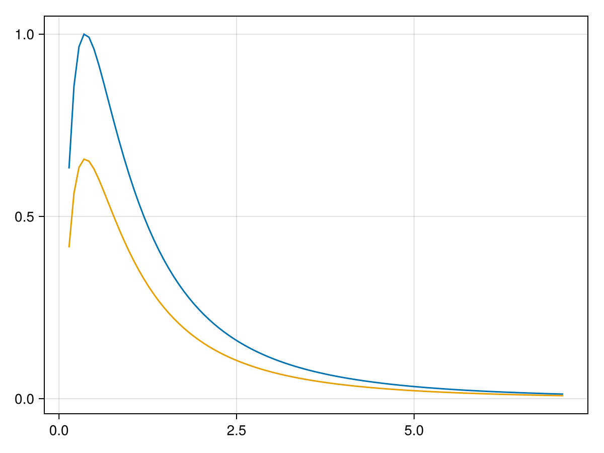

FigureHelpers.density_dist — Function

density_dist(d::UnivariateDistribution; ...)
density_dist!(ax, d::UnivariateDistribution; ...)

Plot density of univariate distribution, d. The first variant produced a figure. The second plots into given Axis.

Keyword arguments

normalize = false: to scale y-axis to 1 for comparing densities with different spread
prange = (0.025, 0.975): truncate x-axis to focus on main mass of the density

source

Plots of MCMCChains

Overview: combined trace-plot with density plot.

For linkaxes=true, all the density plots are on the same x-scale.

using MCMCChains
chn = Chains(rand(500, 2, 3), [:a, :b]);
fig = plot_chn(chn; linkaxes=true)
fig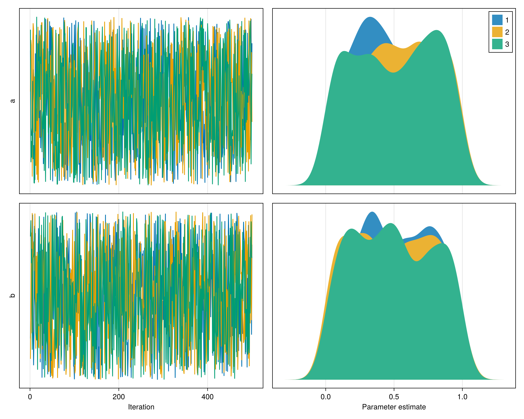

FigureHelpers.plot_chn — Function

plot_chn(fchns::AbstractMCMC.AbstractChains; ... )
plot_chn!(fig::Figure, chns::AbstractMCMC.AbstractChains; ... )

Plot MCMCChain lines and density. The first variant produces a figure, the second variant plots into a matrix-grid of axes into given figure.

Keyword arguments

linkaxes=false: link x-axis across density plots of several chains
param_label="Parameter estimate": x-axis label below lowest density plot
params = names(chns, :parameters): subset of parameters to plot

source

Tailored density plot

Supports more keyword arguments to adjust color and labels.

using MCMCChains
chn = Chains(rand(500, 2, 3), [:a, :b]);
fig = density_params(chn, ["a","b"], labels=["bla","foo","bar"]);
fig[:, 2] = Legend(fig, content(fig[1,1]), "Chain", framevisible = false)
fig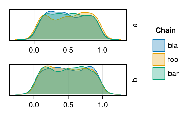

FigureHelpers.density_params — Function

hdensity_params(chns, pars=names(chns, :parameters); 
    makie_config::MakieConfig=MakieConfig(), 
    fig = figure_conf(cm2inch.((8.3,8.3/1.618)); makie_config), 
    column = 1, xlims=nothing, 
    labels=nothing, colors = nothing, ylabels = nothing, normalize = false, 
    kwargs_axis = repeat([()],length(pars)), 
    prange = (0.025, 0.975), # do not extend x-scale to outliers
    kwargs...
)
histogram_params(chns, ...)

Density/Histogram of several variables of a 3D array, i.e. MCMCChain.

Arguments

column: The axis-grid column into which to plot
xlims: indexable of length(pars), providing (lower,upper) bounds tuple for x-limits
labels, colors: names (default chain number) and colors (default palette) of the chains
ylabels: column labels (default parameter names)
normalize: if true, scale all chain densities to maximum one for each row
kwargs_axis: indexable of keyword arguments to axis for each parameter
prange: bounds to the x-axis in percentiles
kwargs: further keyword arguments to lines! (if normalize) or density!

Returns the created figure.

The density plot gives wrong impressions, if probability mass is concentrated at the borders, therefore provide an histogram equivalent.

source