Author Bernhard AhrensAuthor Lazaro Alonso

Getting Started

This page demonstrates how to use EasyHybrid to create a hybrid model for ecosystem respiration. You will become familiar with the following concepts:

Key concepts

1. Process-based Model: The RbQ10 function represents a classical Q10 model for respiration with base respiration rb and Q10 which describes the factor by respiration is increased for a 10 K change in temperature.

2. Neural Network: Learns to predict the basal respiration parameter rb from environmental conditions.

3. Hybrid Integration: Combines the neural network predictions with the process-based model to produce final outputs.

4. Parameter Learning: Some parameters (like Q10) can be learned globally, while others (like rb) are predicted per sample.

The framework automatically handles the integration between neural networks and mechanistic models, making it easy to leverage both data-driven learning and domain knowledge.

Installation

Install Julia v1.10 or above. EasyHybrid.jl is available through the Julia package manager. You can enter it by pressing ] in the REPL and then typing add EasyHybrid. Alternatively, you can also do

import Pkg
Pkg.add("EasyHybrid")

Quickstart

1. Setup and Data Loading

Load package and synthetic dataset

using EasyHybrid

ds = load_timeseries_netcdf("https://github.com/bask0/q10hybrid/raw/master/data/Synthetic4BookChap.nc")
ds = ds[1:20000, :]  # Use subset for faster execution
first(ds, 5)

5×6 DataFrame

Row	time	sw_pot	dsw_pot	ta	reco	rb
	DateTime	Float64?	Float64?	Float64?	Float64?	Float64?
1	2003-01-01T00:15:00	109.817	115.595	2.1	0.844741	1.42522
2	2003-01-01T00:45:00	109.817	115.595	1.98	0.840641	1.42522
3	2003-01-01T01:15:00	109.817	115.595	1.89	0.837579	1.42522
4	2003-01-01T01:45:00	109.817	115.595	2.06	0.843372	1.42522
5	2003-01-01T02:15:00	109.817	115.595	2.09	0.844399	1.42522

2. Define the Process-based Model

RbQ10 model: Respiration model with Q10 temperature sensitivity

function RbQ10(;ta, Q10, rb, tref = 15.0f0)
    reco = rb .* Q10 .^ (0.1f0 .* (ta .- tref))
    return (; reco, Q10, rb)
end

RbQ10 (generic function with 1 method)

3. Configure Model Parameters

Parameter specification: (default, lower_bound, upper_bound)

parameters = (
    rb  = (3.0f0, 0.0f0, 13.0f0),  # Basal respiration [μmol/m²/s]
    Q10 = (2.0f0, 1.0f0, 4.0f0),   # Temperature sensitivity - describes factor by which respiration is increased for 10 K increase in temperature [-]
)

(rb = (3.0f0, 0.0f0, 13.0f0), Q10 = (2.0f0, 1.0f0, 4.0f0))

4. Construct the Hybrid Model

Define input variables

forcing = [:ta]                    # Forcing variables (temperature)
predictors = [:sw_pot, :dsw_pot]   # Predictor variables (solar radiation)
target = [:reco]                   # Target variable (respiration)

1-element Vector{Symbol}:
 :reco

Parameter classification as global, neural or fixed (difference between global and neural)

global_param_names = [:Q10]        # Global parameters (same for all samples)
neural_param_names = [:rb]         # Neural network predicted parameters

1-element Vector{Symbol}:
 :rb

Construct hybrid model

hybrid_model = constructHybridModel(
    predictors,               # Input features
    forcing,                  # Forcing variables
    target,                   # Target variables
    RbQ10,                    # Process-based model function
    parameters,               # Parameter definitions
    neural_param_names,       # NN-predicted parameters
    global_param_names,       # Global parameters
    hidden_layers = [16, 16], # Neural network architecture
    activation = swish,       # Activation function
    scale_nn_outputs = true,  # Scale neural network outputs
    input_batchnorm = true    # Apply batch normalization to inputs
)

Neural Network:
    Chain(
        layer_1 = BatchNorm(2, affine=false, track_stats=true),
        layer_2 = Dense(2 => 16, swish),              # 48 parameters
        layer_3 = Dense(16 => 16, swish),             # 272 parameters
        layer_4 = Dense(16 => 1),                     # 17 parameters
    )         # Total: 337 parameters,
              #        plus 5 states.
Predictors: [:sw_pot, :dsw_pot]
Forcing: [:ta]
Neural parameters: [:rb]
Global parameters: [:Q10]
Fixed parameters: Symbol[]
Scale NN outputs: true
Parameter defaults and bounds:
    HybridParams{typeof(Main.RbQ10)}(
    ┌─────┬─────────┬───────┬───────┐
    │     │ default │ lower │ upper │
    ├─────┼─────────┼───────┼───────┤
    │  rb │     3.0 │   0.0 │  13.0 │
    │ Q10 │     2.0 │   1.0 │   4.0 │
    └─────┴─────────┴───────┴───────┘
    )

5. Train the Model

out = train(
    hybrid_model,
    ds,
    ();
    nepochs = 100,               # Number of training epochs
    batchsize = 512,             # Batch size for training
    opt = RMSProp(0.001),        # Optimizer and learning rate
    monitor_names = [:rb, :Q10], # Parameters to monitor during training
    yscale = identity,           # Scaling for outputs
    patience = 30,               # Early stopping patience
    show_progress=false,
)

  train_history: (101, 2)
    mse  (reco, sum)
    r2   (reco, sum)
  val_history: (101, 2)
    mse  (reco, sum)
    r2   (reco, sum)
  ps_history: (101, 2)
    ϕ        ()
    monitor  (train, val)
  train_obs_pred: 16000×3 DataFrame
    reco, index, reco_pred
  val_obs_pred: 4000×3 DataFrame
    reco, index, reco_pred
  train_diffs: 
    Q10         (1,)
    rb          (16000,)
    parameters  (rb, Q10)
  val_diffs: 
    Q10         (1,)
    rb          (4000,)
    parameters  (rb, Q10)
  ps: 
    ps   (layer_1, layer_2, layer_3, layer_4)
    Q10  (1,)
  st: 
    st     (layer_1, layer_2, layer_3, layer_4)
    fixed  ()
  best_epoch: 
  best_loss: 

6. Check Results

Evolution of train and validation loss

using CairoMakie
EasyHybrid.plot_loss(out, yscale = identity)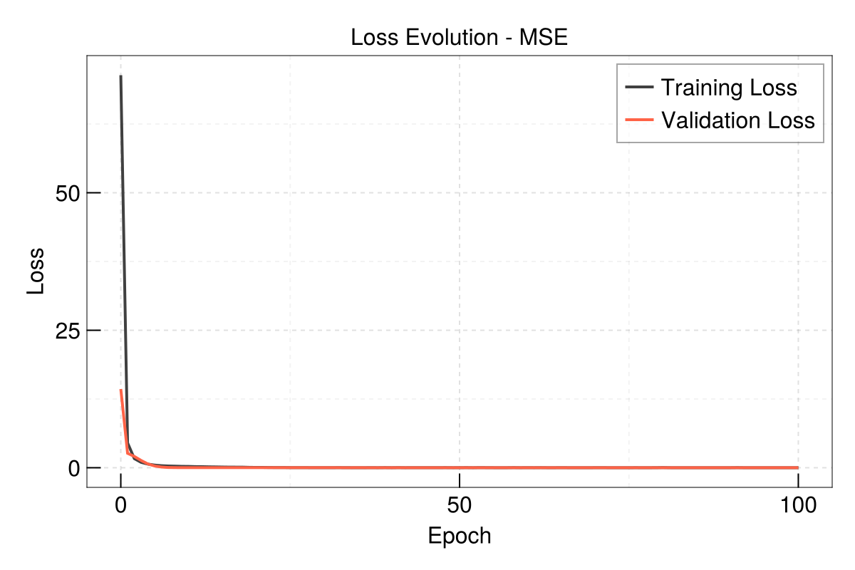

Check results - what do you think - is it the true Q10 used to generate the synthetic dataset?

out.train_diffs.Q10

1-element Vector{Float32}:
 1.4999903

Quick scatterplot - dispatches on the output of train

EasyHybrid.poplot(out)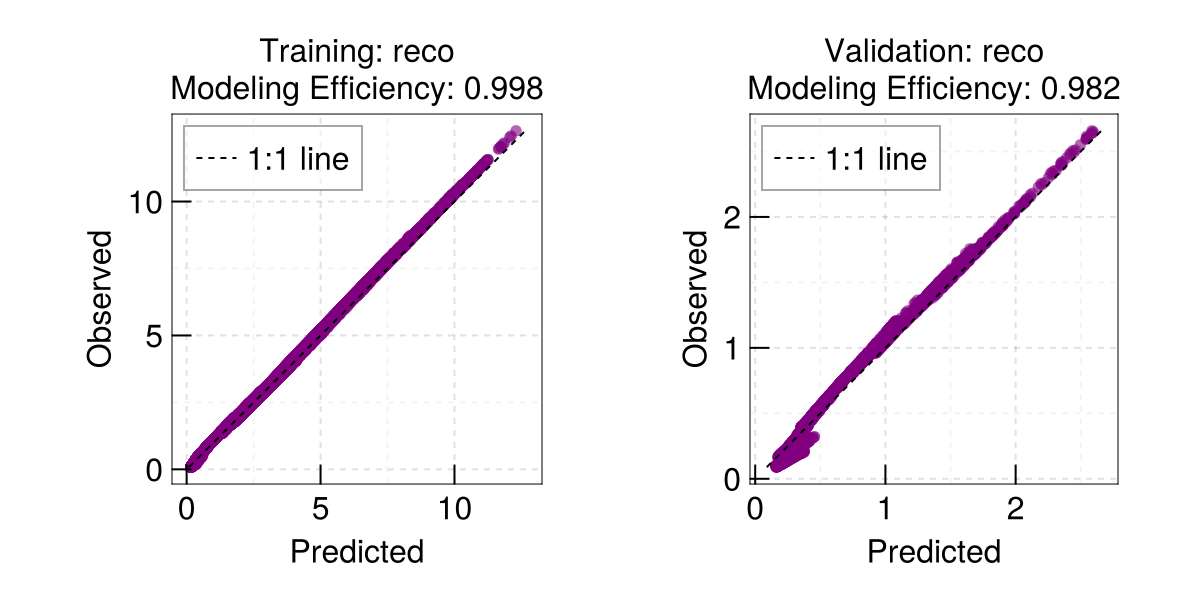

More Examples

Check out the projects/ directory for additional examples and use cases. Each project demonstrates different aspects of hybrid modeling with EasyHybrid.