nicefigs

Publication-grade, modular matplotlib plotting for geoscience.

nicefigs is a thin, composable layer on top of matplotlib. It gives you a single consistent house style (sans-serif, journal-like), physical figure sizing that keeps fonts consistent across every panel, and a toolbox of geoscience-ready plots: global/regional maps, ternary maps & scatters, image grids, tight colorbars, KDE agreement plots, model-comparison violins, timeseries, and map animations.

Design philosophy

One consistent house style. A small, explicit Theme dataclass bundles font sizes, line widths, and colours. Call nicefigs.set_theme("paper") once and every helper — maps, scatter plots, heatmaps, timeseries — renders with matching fonts, tick sizes, and spine weights.

Physical figure sizing. You almost never want to think in inches. You want "a single-column figure" or "half the text width". Because font sizes live in points and figure sizes live in inches, nicefigs.figure / nicefigs.subplots solve the figure size from a named physical target (width="single", width="half", ...) and an aspect ratio. The rendered figure lands at exactly the requested physical size, with fonts at exactly the theme's point sizes — so a multi-panel paper figure looks consistent whether one panel is a map and another is a scatter plot.

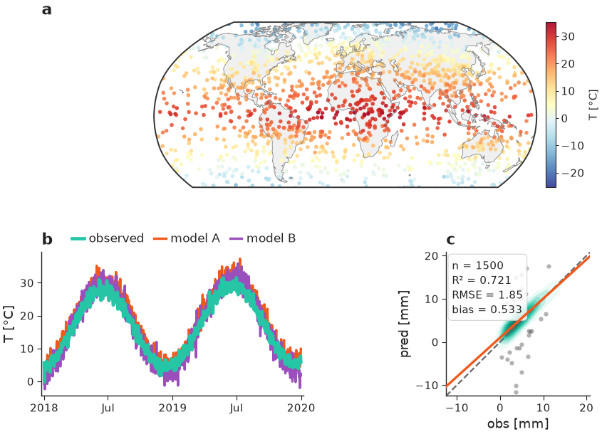
Modular, composable helpers. Every plotting function accepts an existing ax (or fig) where it makes sense, so you can drop nicefigs pieces into your own matplotlib layouts — a GridSpec, a plt.subplots grid, an inset axes — rather than being handed a fixed figure you have to fight with. The composite figure example shows a map, a timeseries, and an agreement plot composed into one GridSpec, all sharing one theme and one physical width.

Install

pip install nicefigs

# with cartopy-backed map projections
pip install "nicefigs[maps]"

# with xarray input helpers
pip install "nicefigs[xarray]"

# both
pip install "nicefigs[all]"

A first example

The figure above is built from three independently composable pieces — a map, a timeseries, and an agreement plot — arranged in a GridSpec, all at one consistent physical width. See it fully worked through in the Gallery and Quickstart.

import nicefigs as nf
from nicefigs import data

nf.set_theme("paper")

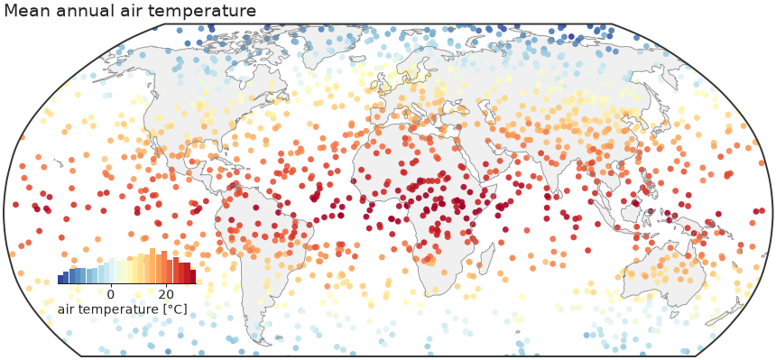
lon, lat, temp = data.global_points(field="temperature")
fig, ax, m = nf.map(
    lon, lat, temp,
    cmap="RdYlBu_r",
    colorbar_label="air temperature [°C]",
    title="Mean annual air temperature",
)
nf.save(fig, "figures/global_map", formats=("pdf", "png"))

Continue to the Quickstart or browse the full Gallery for every plot family, or jump straight to the API Reference.