Maps

map() draws values at longitude/latitude on a Robinson-projected world map with Antarctica cropped, a light land backdrop, coastlines and an inset histogram that doubles as the colorbar. It returns (fig, ax, mappable). With cartopy installed (pip install "nicefigs[maps]") the map is projected; without it, every map helper falls back to a plain equirectangular axes. The examples set the house style with nf.set_theme("paper"); see Styling & themes.

Mapping scattered points

Pass 1-D lon, lat and values; below 5000 points map scatters them:

import nicefigs as nf
from nicefigs import data

nf.set_theme("paper")

lon, lat, temp = data.global_points(field="temperature")
fig, ax, mappable = nf.map(
    lon, lat, temp,
    cmap="RdYlBu_r",
    colorbar_label="air temperature [°C]",
    title="Mean annual air temperature",
)
print(type(mappable).__name__, len(temp))

PathCollection 1729

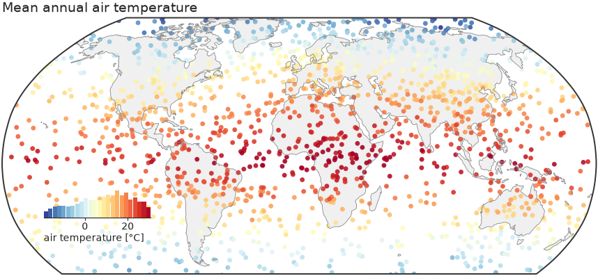
Colour limits come from the 2nd and 98th percentiles (robust=True), so a few extreme stations do not wash out the scale.

Bin-averaging dense data

kind picks "scatter", "binned" or "auto" (binned above 5000 points). kind="binned" averages onto a bin_deg grid; diverging=True picks a diverging colormap with limits symmetric about center (default 0), the right choice for anomalies:

import nicefigs as nf
from nicefigs import data

nf.set_theme("paper")

lon, lat, anom = data.global_points(n=9000, field="anomaly")
fig, ax, mappable = nf.map(
    lon, lat, anom,
    kind="binned", diverging=True, bin_deg=2.5,
    colorbar_label="temperature anomaly [K]",
)
vmin, vmax = mappable.get_clim()
print(f"{vmin:.2f} {vmax:.2f}")

-4.59 4.59

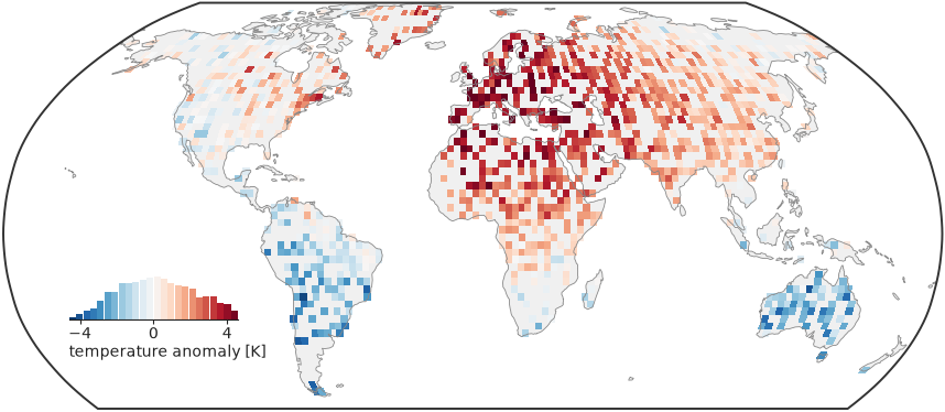
The limits are symmetric, so zero sits on the colormap's neutral centre. A global binned map drops bins whose centre is at sea; pass clip_ocean=False for data measured over the ocean.

Choosing a projection and extent

projection is one of "robinson" (default), "platecarree", "mollweide", "equalearth", "orthographic" or "nearside", resolved by make_map_axes(); an unknown name raises ValueError. extent=(west, east, south, north) zooms to a region and replaces the default Antarctica crop (ANTARCTICA_CUTOFF_EXTENT):

import nicefigs as nf
from nicefigs import data

nf.set_theme("paper")

lon, lat, field = data.regional_grid(res=0.25)
fig, ax, mappable = nf.map(
    lon, lat, field,
    extent=(5, 20, 45, 55),
    projection="platecarree",
    diverging=True, inset_hist=False, cbar=True, borders=True,
    colorbar_label="soil-moisture anomaly [m³ m⁻³]",
)
print(field.shape)

(40, 60)

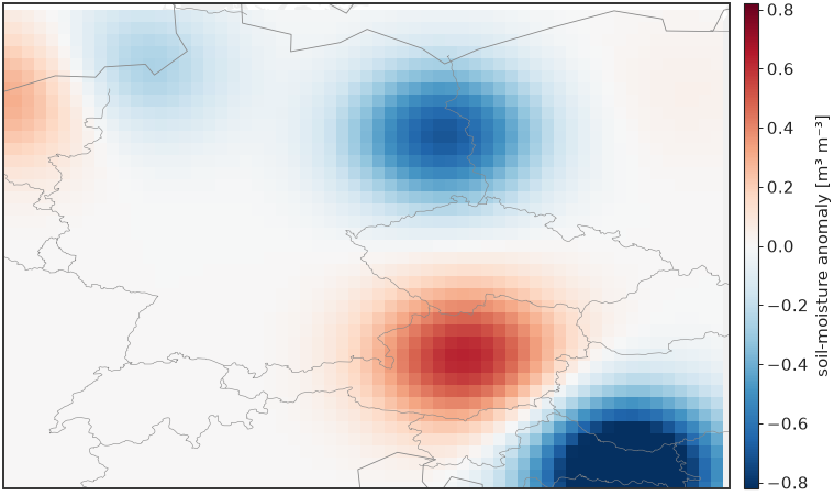
A 2-D field is drawn as a raster; a regional map usually wants a slim colorbar (cbar=True) rather than the inset histogram.

Mapping gridded and unstructured data

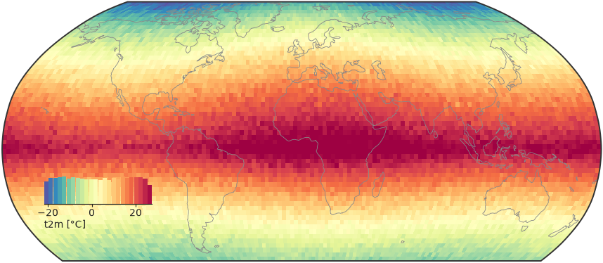
map dispatches on its input. A 2-D values array on a regular grid goes to raster_map() (pcolormesh); a DataArray with recognisable longitude/latitude coordinates is unpacked by from_xarray() first:

import nicefigs as nf
from nicefigs import data

nf.set_theme("paper")

da = data.global_dataarray()
lon, lat, field = nf.from_xarray(da)
fig, ax, mappable = nf.map(da, cmap="Spectral_r", colorbar_label="t2m [°C]")
print(da.dims, field.shape)

('lat', 'lon') (72, 144)

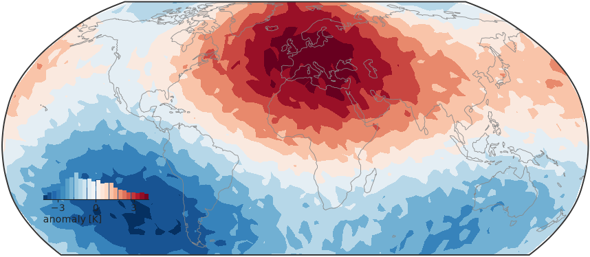
For points on an unstructured or icosahedral mesh, kind="tri" triangulates them in projected coordinates and draws them with tri_map() (tricontourf, or "tripcolor"). Triangles that would span the antimeridian or wrap over a pole are masked:

import nicefigs as nf
from nicefigs import data

nf.set_theme("paper")

lon, lat, values = data.icosahedral_field(n=3000)
fig, ax, mappable = nf.map(lon, lat, values, kind="tri", diverging=True,
                           colorbar_label="anomaly [K]")

Mapping class labels

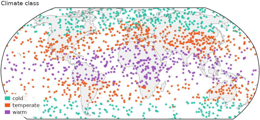
categorical_map() draws a class label per point — a land-cover code, a cluster id, a mask — in discrete colours with a patch legend instead of a colorbar. Through map, pass kind="categorical" and the ordered categories:

import numpy as np

import nicefigs as nf
from nicefigs import data

nf.set_theme("paper")

lon, lat, temp = data.global_points(field="temperature")
codes = np.digitize(temp, [5.0, 20.0])  # 0 cold, 1 temperate, 2 warm
fig, ax, mappable = nf.map(
    lon, lat, codes, kind="categorical",
    categories=["cold", "temperate", "warm"],
    title="Climate class",
)
print([t.get_text() for t in ax.get_legend().get_texts()])

['cold', 'temperate', 'warm']

A sequence of names reads codes as 0..n-1; a {code: name} mapping takes arbitrary codes. Colours default to qualitative() and can be set with colors. Codes outside categories and non-finite coordinates are dropped. Above 5000 points the cloud is gridded by majority vote per cell, since the mean of class codes is meaningless; ties go to the category listed first.

Note

Class codes carry their own discrete norm, so vmin, vmax, robust and diverging are ignored for kind="categorical", and no colorbar or inset histogram is drawn.

Composing map panels

The layer helpers — scatter_map(), binned_map(), raster_map, tri_map and categorical_map — draw onto a map axes you pass as ax and return (ax, mappable); the cartopy CRS is detected from the axes. Build the axes with make_map_axes(), add land and coastlines with draw_background(), and share one colorbar across panels with colorbar():

import nicefigs as nf
from nicefigs import data

nf.set_theme("paper")
fig = nf.figure(width="full", aspect=0.32)
lon, lat, anom = data.global_points(field="anomaly")
for i in range(2):
    ax, ccrs = nf.make_map_axes(fig, (1, 2, i + 1))
    nf.draw_background(ax, ccrs)
    _, mappable = nf.scatter_map(lon, lat, anom * (i + 1), ax=ax, cmap="RdBu_r",
                                 vmin=-4, vmax=4, size=3)
    ax.set_title(f"scenario {i + 1}")
nf.colorbar(mappable, fig.axes, label="anomaly [K]", location="bottom", shrink=0.5)

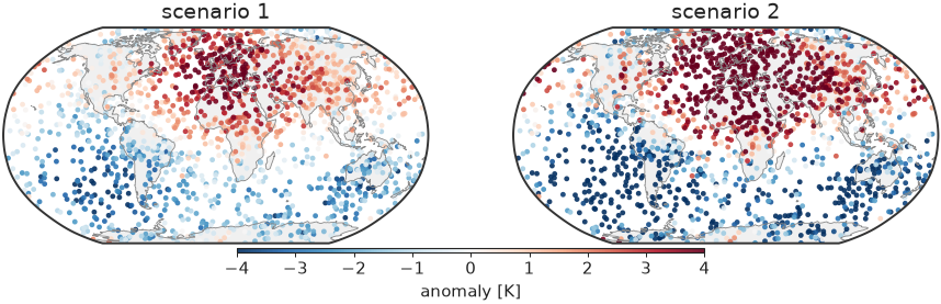
Both panels share fixed limits, so one colorbar reads for both.

Docking the histogram colorbar

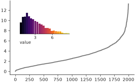
inset_histogram_colorbar() is the histogram map docks in the empty South Pacific: a histogram of the mapped values coloured by the same colormap, so it shows both the colour scale and the data distribution. Call it on any axes; bounds places it in axes fractions:

import numpy as np

import nicefigs as nf

nf.set_theme("paper")

values = np.random.default_rng(0).gamma(2.0, 1.5, 2000)
fig, ax = nf.subplots(width="half", aspect=0.6)
ax.plot(np.sort(values), color="0.5")
nf.inset_histogram_colorbar(ax, values, cmap="inferno", bounds=(0.08, 0.55, 0.4, 0.3),
                            label="value")

Ternary maps

For a three-part composition per point, such as land-use fractions, ternary_map() colours each point by a barycentric blend of three corner colours and adds a triangular legend:

import nicefigs as nf
from nicefigs import data

nf.set_theme("paper")

lon, lat, _ = data.global_points(n=600, land_bias=False)
comp, _ = data.ternary_points(n=600)
fig, ax = nf.ternary_map(lon, lat, comp, labels=("Forest", "Crop", "Urban"),
                         size=7, title="Dominant land use")
print(comp.shape, comp.sum(axis=1).min().round(6))

(600, 3) 1.0

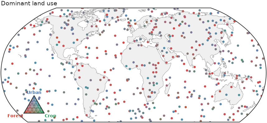
See Colormaps & palettes for the corner palettes shared by every ternary helper.