Colormaps & palettes

Every colour helper resolves by name: cmap() for continuous colormaps, categorical() for class-code rasters, qualitative() and artist_palette() for lists of distinct colours. Unknown names raise KeyError. Examples that draw set the house style with nf.set_theme("paper").

Resolving continuous colormaps

DEFAULTS maps a kind of data to a colormap. cmap(name, n=None) resolves such a kind, a matplotlib name (case-insensitive) or a Colormap, and resamples it to n levels if asked:

import nicefigs as nf

print(nf.DEFAULTS["diverging"], nf.DEFAULTS["intensity"])
print(nf.cmap("spectral_r").name)
print(nf.cmap("diverging").name)
print(nf.cmap("viridis", n=8).N)

RdBu_r inferno
Spectral_r
RdBu_r
8

Name a kind ("diverging", "sequential", "cyclic") rather than a colormap, and every figure of one kind changes together.

Centring diverging data

For anomalies centred on a meaningful value, symmetric_limits() returns (-m, m) from a robust percentile of |values|, robust_limits() returns percentile limits, and diverging_norm() builds a TwoSlopeNorm around center:

import numpy as np

import nicefigs as nf

anomaly = np.random.default_rng(0).normal(0.3, 1.0, 5000)
lo, hi = nf.symmetric_limits(anomaly)
norm = nf.diverging_norm(lo, hi, center=0.0)
print(f"{lo:.2f} {hi:.2f}", f"{norm(0.0):.2f}")
print([f"{v:.2f}" for v in nf.robust_limits(anomaly)])

-2.42 2.42 0.50
['-1.71', '2.34']

Zero maps to the middle of the colormap even though the data are skewed. map(..., diverging=True) uses the same limits.

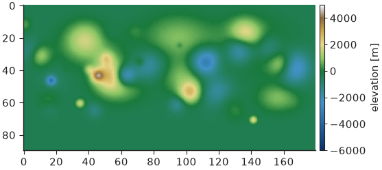
Elevation colormap

elevation_cmap() returns a hypsometric (cmap, norm) pair — blues below sea_level, green to tan to white above — with the norm placing sea_level exactly at the land/sea break for any vmin/vmax:

import nicefigs as nf
from nicefigs import data

nf.set_theme("paper")

elevation = data.elevation_field(shape=(90, 180))
cmap, norm = nf.elevation_cmap(vmin=-6000, vmax=5000)
fig, ax = nf.subplots(width="half", aspect=0.55)
im = ax.imshow(elevation, cmap=cmap, norm=norm)
nf.colorbar(im, ax, label="elevation [m]")
print(f"{norm(0.0):.3f}")

0.545

Banded scorecard colormap

scorecard_diverging_cmap() returns a (cmap, norm) pair for percent differences: 11 discrete, quasi-logarithmic bands over SCORECARD_DIVERGING_BOUNDARIES, a light-grey centre band, and distinct colours beyond ±50 %:

import numpy as np

import nicefigs as nf

nf.set_theme("paper")

cmap, norm = nf.scorecard_diverging_cmap()
print(nf.SCORECARD_DIVERGING_BOUNDARIES)
pct_diff = np.random.default_rng(1).normal(0, 15, (4, 6))
fig, ax = nf.subplots(width="half", aspect=0.6)
im = ax.imshow(pct_diff, cmap=cmap, norm=norm)
ax.set_axis_off()
nf.colorbar(im, ax, extend="both", label="difference [%]")

[-50, -20, -10, -5, -2, -1, 1, 2, 5, 10, 20, 50]

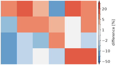
The narrow bands near zero keep differences of a few percent apart, where a linear ±100 % scale would render them all as near-white.

Land-cover palettes

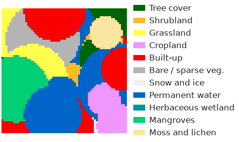
categorical(name) returns a Categorical — class codes mapped to names and colours — from CATEGORICAL: "esa_worldcover", "esri_lulc" and "modis_igbp". It gives a (cmap, norm) pair for imshow, an RGB image, and legend patches:

import nicefigs as nf
from nicefigs import data

nf.set_theme("paper")

lc = nf.categorical("esa_worldcover")
codes = data.landcover_patch(size=64)
cmap, norm = lc.cmap_norm()
fig, ax = nf.subplots(width="half", aspect=0.6)
ax.imshow(codes, cmap=cmap, norm=norm)
ax.set_axis_off()
ax.legend(handles=lc.legend_handles(), loc="center left", bbox_to_anchor=(1.0, 0.5),
          frameon=False, fontsize=6)
print(sorted(nf.CATEGORICAL), lc.to_rgb(codes).shape)

['esa_worldcover', 'esri_lulc', 'modis_igbp'] (64, 64, 3)

Qualitative and artist palettes

qualitative(n, palette="nice") returns n distinct colours, cycling past the palette length. The default "nice" palette (NICE) is a bright teal ahead of colours sampled from David Hockney's A Bigger Grand Canyon; it is also every theme's colour cycle. "bright", "muted" and "high_contrast" are Paul Tol's colour-blind-safe palettes, and ARTIST_PALETTES adds palettes from MetBrewer and MoMAColors:

import nicefigs as nf

print(nf.qualitative(3))
print(nf.qualitative(3, "bright"))
print(nf.artist_palette("hiroshige", 4))
print(len(nf.ARTIST_PALETTES))

['#25c5a6', '#ef5a1c', '#9a4fbc']
['#4477AA', '#EE6677', '#228833']
['#e76254', '#ef8a47', '#f7aa58', '#ffd06f']
27

Each artist palette is also registered as a continuous colormap, built by artist_cmap() and resolvable through cmap:

import numpy as np

import nicefigs as nf

nf.set_theme("paper")

fig, axes = nf.subplots(3, 1, width="half", aspect=0.45, hspace=1.2)
gradient = np.linspace(0, 1, 256)[None, :]
for ax, name in zip(axes, ["nice_teal", "hockney_canyon", "hiroshige"]):
    ax.imshow(gradient, aspect="auto", cmap=nf.cmap(name))
    ax.set_title(name, loc="left", fontsize=6)
    ax.set_axis_off()

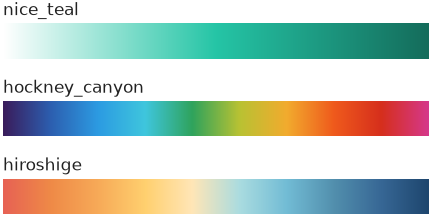
nice_teal, nice_orange and nice_purple are white-to-colour ramps for density shading in the house colours.

Ternary colour encoding

A composition (a, b, c) with a + b + c = 1 becomes a colour by blending three corner colours barycentrically with ternary.color(). It underlies ternary_scatter(), ternary_map() and ternary_image(). corners takes three colours or a name from TERNARY_PALETTES:

import nicefigs as nf
from nicefigs import data

nf.set_theme("paper")

print(sorted(nf.TERNARY_PALETTES))
comp, _ = data.ternary_points(n=300)
ax, _ = nf.ternary_scatter(comp, corners="bright", labels=("A", "B", "C"))

['bright', 'default', 'muted', 'prevalence', 'warm']

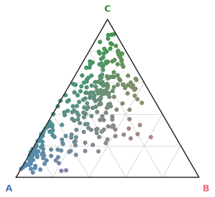
A pure component takes its corner colour; an even mix tends to grey.

Bivariate colormaps

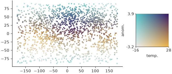
When two continuous variables share one plot, a 2-D colormap encodes both. colormaps2d maps (x, y) in [0, 1]² to RGB with bivariate_cmap() (four blended corners), hsv_cmap() (hue × saturation) or flat_cmap() (constant CIE-Lab lightness), each with a matching legend. normalize01() rescales raw values (5th–95th percentile by default) and returns the range for the legend ticks:

import nicefigs as nf
from nicefigs import data
from nicefigs.colormaps2d import normalize01

nf.set_theme("paper")

lon, lat, temp = data.global_points(field="temperature")
_, _, anom = data.global_points(field="anomaly")
tx, trange = normalize01(temp)
ay, arange_ = normalize01(anom)
fig, ax = nf.subplots(width="half", aspect=0.6)
ax.scatter(lon, lat, c=nf.bivariate_cmap(tx, ay), s=3, linewidths=0)
iax = ax.inset_axes([1.12, 0.3, 0.3, 0.5])
nf.bivariate_legend(iax, x_label="temp.", y_label="anom.", x_range=trange, y_range=arange_)

Note

A bivariate colormap is hard to read precisely; use it to show where two variables co-occur, and give exact values in a separate panel.