Plots

This page covers the plotting helpers beyond maps: images, scatter and agreement plots, time series, model comparisons, rankings, scorecards, vertical sections and Hovmöller diagrams. Every helper takes ax=None and creates a figure when it is missing; see the calling conventions for what each returns.

Showing images and heatmaps

image() shows an intensity array coloured by cmap, or an (H, W, 3|4) colour image, without ticks. stretch=True contrast-stretches a colour image per channel. heatmap() adds row and column labels and, with annotate=True, the value of each cell.

import nicefigs as nf
from nicefigs import data

nf.set_theme("paper")
fig, (ax_img, ax_hm) = nf.subplots(1, 2, width="full", panel_aspect=0.8, wspace=0.3)
nf.image(data.rgb_patch(), stretch=True, title="RGB patch", ax=ax_img)
nf.heatmap(
    data.heatmap_matrix(shape=(5, 6)),
    row_labels=list("ABCDE"),
    col_labels=[f"c{j}" for j in range(6)],
    annotate=True,
    ax=ax_hm,
)

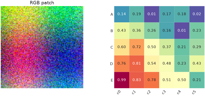
A three-channel array is drawn as colour; a two-dimensional array is drawn with cmap.

image_grid() lays out several images with one shared colour scale and colorbar. colorbar_mode is "single" (default), "row", "each" or "none"; shared_scale=False gives each image its own limits.

import nicefigs as nf
from nicefigs import data

nf.set_theme("paper")
images = [data.regional_grid(seed=i)[2] for i in range(6)]
fig, axes = nf.image_grid(
    images,
    nrows=2,
    ncols=3,
    width="full",
    cmap="Spectral_r",
    colorbar_label="value",
    titles=[f"member {i + 1}" for i in range(6)],
)
nf.label_panels(axes)

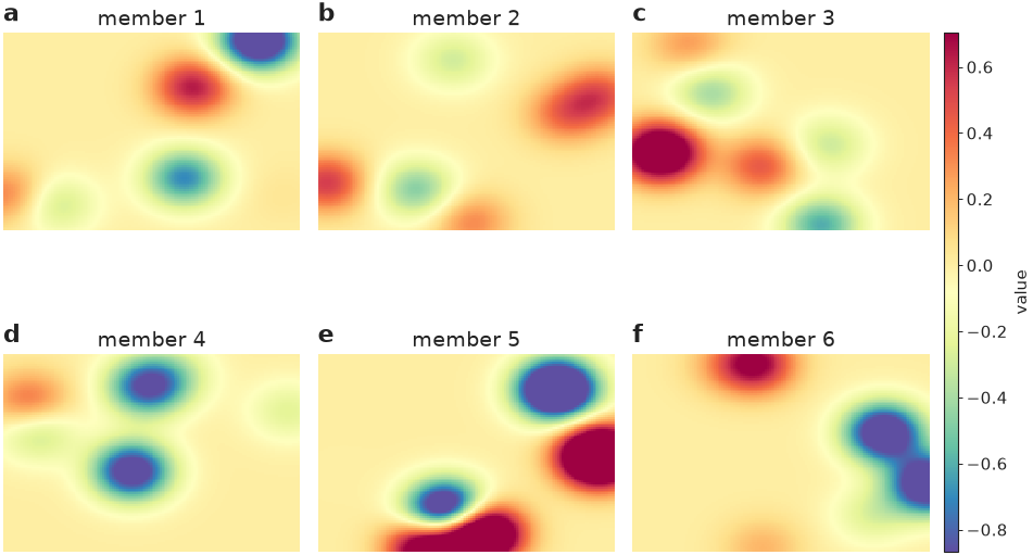
All six panels share one colorbar, so equal colours mean equal values.

For land-cover rasters, pass a Categorical palette's .to_rgb() to image(); see Colormaps & palettes.

Scatter plots with encodings

scatter() maps extra variables onto marker shape (a categorical group), size (size, scaled into size_range) and colour (a continuous hue, or group), and builds a legend for each.

import nicefigs as nf
from nicefigs import data

nf.set_theme("paper")
d = data.scatter_bubbles(n=140)
ax, artists = nf.scatter(
    d["x"], d["y"], group=d["group"], size=d["size"], size_label="area [km²]", alpha=0.8
)
nf.set_labels(ax, "predictor", "response")
print(sorted(artists))

['A', 'B', 'C']

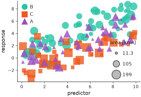
With group, the second return value maps each group to its collection. hue=values, colorbar=True colours by a continuous variable instead; xerr/yerr add error bars and point_labels with label_top=n labels the n most extreme points.

Agreement plots

agreement() compares predictions with observations: a density of the point cloud (density="kde", "hexbin" or "hist"), a dashed 1:1 line, outliers as faint points, a regression line and a metrics box. It returns the metrics as a dict.

import nicefigs as nf
from nicefigs import data

nf.set_theme("paper")
obs, pred = data.xy_agreement()
ax, stats = nf.agreement(
    obs, pred, xlabel="observed runoff", ylabel="predicted runoff", units="mm d⁻¹", width="half"
)
print({k: round(float(v), 3) for k, v in stats.items()})

{'slope': 0.906, 'intercept': 1.001, 'r2': 0.721, 'rmse': 1.846, 'bias': 0.533, 'n': 1500.0}

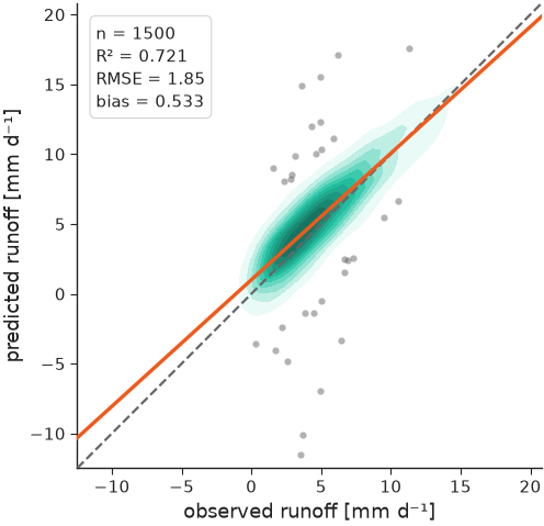
The printed metrics are the ones in the box on the plot.

Time series

timeseries() plots named series against dates and picks date ticks for the span. bands shades an interval per series and highlight draws one series thicker and on top.

import nicefigs as nf
from nicefigs import data

nf.set_theme("paper")
dates, series = data.timeseries(n_days=365)
model = series["model A"]
ax = nf.timeseries(
    dates,
    series,
    bands={"model A": (model - 2.0, model + 2.0)},
    highlight="observed",
    ylabel="air temperature",
    yunits="degC",
    width="full",
)

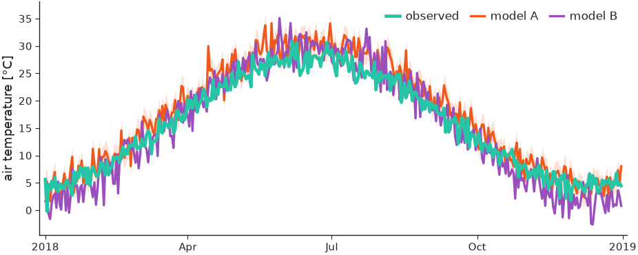
The observed series sits on top of the two models; model A carries its band.

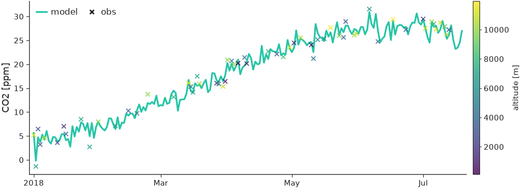
Sparse observations go in obs=(dates, values) and are drawn as markers. obs_hue colours them by a third variable, with obs_colorbar=True for its colorbar:

import numpy as np

import nicefigs as nf
from nicefigs import data

nf.set_theme("paper")
dates, series = data.timeseries(n_days=200, series=["model"])
rng = np.random.default_rng(0)
idx = np.sort(rng.choice(len(dates), 60, replace=False))
obs_dates = [dates[i] for i in idx]
obs_vals = series["model"][idx] + rng.normal(0, 1, 60)
ax = nf.timeseries(
    dates,
    series,
    obs=(obs_dates, obs_vals),
    obs_hue=rng.uniform(0, 12000, 60),
    obs_cmap="viridis",
    obs_hue_label="altitude [m]",
    obs_colorbar=True,
    ylabel="CO2",
    yunits="ppm",
    width="full",
)

styles sets per-series line styles and annotation writes a short note in the panel, which suits small multiples built with facet() (see Figures & sizing).

Comparing models

model_comparison() takes {metric: {model: values}}, or {metric: {model: {group: values}}} for a second split such as timescale, and draws one panel per metric with a violin (kind="violin"), box ("box") or strip ("strip") per model.

import nicefigs as nf
from nicefigs import data

nf.set_theme("paper")
scores = data.model_scores()["scores"]
fig, axes = nf.model_comparison(
    scores, group_label="timescale", kind="box", metric_units={"RMSE": "mm"}
)
print(len(axes))

3

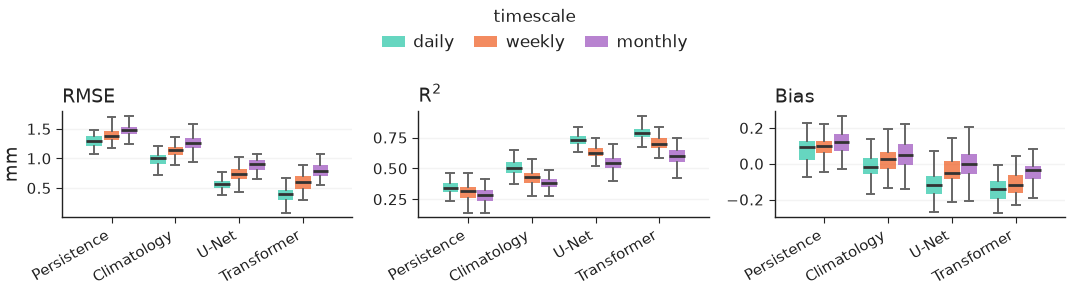
One panel per metric, with the groups dodged inside each model and one shared legend.

taylor() summarises the same question in one diagram: each model sits at its correlation (angle) and standard deviation (radius), with centred-RMS arcs around the reference. Give each model a correlation and either std or std_ratio.

import nicefigs as nf

nf.set_theme("paper")
ax = nf.taylor(
    [
        {"name": "model A", "correlation": 0.93, "std_ratio": 0.98},
        {"name": "model B", "correlation": 0.80, "std_ratio": 1.15},
        {"name": "model C", "correlation": 0.65, "std_ratio": 0.70},
    ],
    width="half",
)

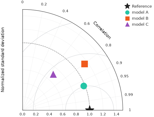
Model A lies closest to the reference star, so it has the smallest centred RMS error.

Ranking and trade-offs

pareto() scatters a trade-off and draws the non-dominated frontier() on top, one per group with frontier_per_group=True. xdirection and ydirection say which way is better; they define the frontier and add arrows to the axis labels.

import nicefigs as nf
from nicefigs import data

nf.set_theme("paper")
d = data.pareto_tradeoff()
ax, _ = nf.pareto(
    d["x"],
    d["y"],
    group=d["group"],
    frontier_per_group=True,
    xdirection="higher_better",
    ydirection="higher_better",
    xlabel="speed",
    ylabel="skill",
)
front = nf.frontier(d["x"], d["y"], xdirection="higher_better", ydirection="higher_better")
print(len(front), "of", len(d["x"]), "points are Pareto-optimal")

14 of 36 points are Pareto-optimal

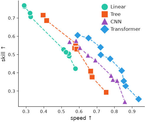
Each group traces its own frontier: no point on it can gain speed without losing skill. baselines={label: y} adds labelled horizontal reference lines.

caterpillar() ranks per-item values with error bars, optionally with a baseline series offset next to each item and a summary annotation.

import nicefigs as nf
from nicefigs import data

nf.set_theme("paper")
s = data.site_metrics(n_sites=16)
ax = nf.caterpillar(
    s["labels"],
    s["bias"],
    err=s["std"],
    groups=s["layer"],
    baseline=s["baseline"],
    baseline_label="reference model",
    value_label="bias",
    value_units="ppmv",
    ref_line=0.0,
)

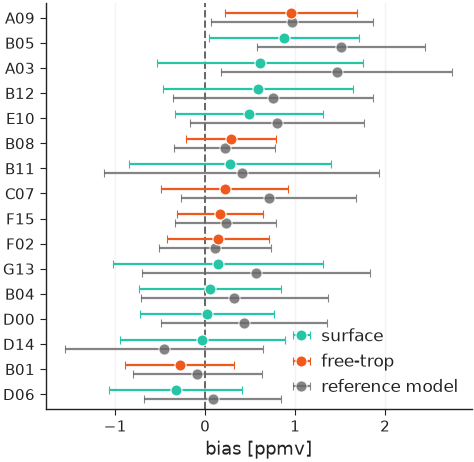
Items are sorted by value, coloured by group, with the reference model's value offset beside each.

Scorecards

scorecard() renders a model × metric table as coloured cells. By default each column is ranked on its own, using each metric's direction from DIRECTIONS, and the best cell per column is outlined.

import numpy as np

import nicefigs as nf
from nicefigs import data

nf.set_theme("paper")
ms = data.model_scores()
values = np.array(
    [[np.mean(ms["scores"][m][model]["daily"]) for m in ms["metrics"]] for model in ms["models"]]
)
ax = nf.scorecard(
    values,
    row_labels=ms["models"],
    col_labels=ms["metrics"],
    direction={"RMSE": "lower_better", "Bias": "target", "R$^2$": "higher_better"},
    col_units={"RMSE": "mm"},
)

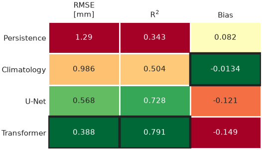
Bias is ranked by closeness to zero, the default target.

To colour cells by their value instead, pass a norm, for example from scorecard_diverging_cmap(). col_groups gaps and titles groups of columns, square=True forces square cells and colorbar=True adds a colorbar.

import numpy as np

import nicefigs as nf

nf.set_theme("paper")
rng = np.random.default_rng(1)
pct_diff = np.vstack([np.zeros(4), rng.normal(-8, 6, (2, 4))])
cmap, norm = nf.scorecard_diverging_cmap()
ax = nf.scorecard(
    pct_diff,
    row_labels=["baseline", "model A", "model B"],
    col_labels=["Z500", "T850", "T2m", "MSL"],
    cmap=cmap,
    norm=norm,
    direction=dict.fromkeys(["Z500", "T850", "T2m", "MSL"], "lower_better"),
    col_groups=["upper air", "upper air", "surface", "surface"],
    square=True,
    cell_format="{:+.0f}",
    colorbar=True,
    colorbar_label="RMSE difference [%]",
)

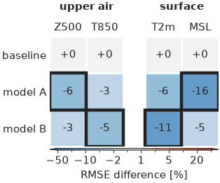
Negative differences, an improvement over the baseline, are blue; the outline marks the lowest value per column.

skill_gap() computes the signed distance of each value from a reference, positive where the value is better. Passing reference= to scorecard colours cells by this gap, so metrics in different units share one scale.

import nicefigs as nf

gap = nf.skill_gap([[0.8, 1.2]], [[1.0, 1.0]], direction=["higher_better", "lower_better"])
print(gap)

[[-0.2 -0.2]]

Both values are 0.2 worse than the reference, whichever way their metric is read.

Bar charts

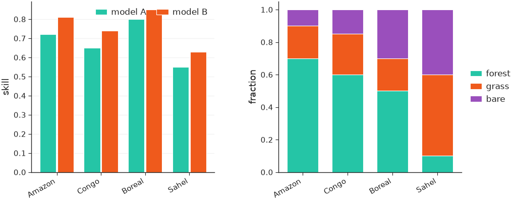
grouped_bars() dodges one bar per (category, series); stacked_bars() stacks the series within each category, as fractions with normalize=True.

import nicefigs as nf

nf.set_theme("paper")
regions = ["Amazon", "Congo", "Boreal", "Sahel"]
fig, (ax_g, ax_s) = nf.subplots(1, 2, width="full", panel_aspect=0.8, wspace=0.35)
nf.grouped_bars(
    regions,
    {"model A": [0.72, 0.65, 0.80, 0.55], "model B": [0.81, 0.74, 0.85, 0.63]},
    value_label="skill",
    rotation=30,
    ax=ax_g,
)
nf.stacked_bars(
    regions,
    {"forest": [0.7, 0.6, 0.5, 0.1], "grass": [0.2, 0.25, 0.2, 0.5], "bare": [0.1, 0.15, 0.3, 0.4]},
    normalize=True,
    rotation=30,
    ax=ax_s,
)

Vertical sections and profiles

cross_section() draws a field over a horizontal and a vertical coordinate, such as latitude × pressure. cross_section_panels() lays out several with shared colorbars: fields named in diff_fields go on a symmetric diverging scale, and log_y=True log-scales the vertical axis.

import nicefigs as nf
from nicefigs import data

nf.set_theme("paper")
cs = data.cross_section_field()
value = cs["value"]
fig, axes = nf.cross_section_panels(
    {"CO₂": value, "anomaly": value - value.mean(axis=0, keepdims=True)},
    cs["lats"],
    cs["levels"],
    diff_fields={"anomaly"},
    value_label="CO₂ [ppm]",
    diff_label="Δ CO₂ [ppm]",
    log_y=True,
)

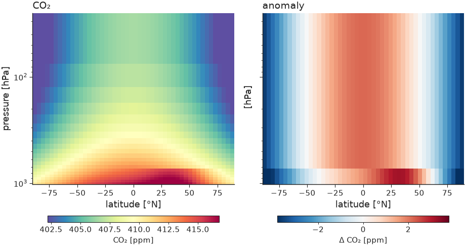
The anomaly panel gets its own diverging colorbar, centred on zero.

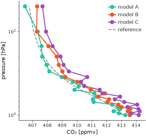
profile() draws value-versus-level profiles with an inverted vertical axis and dashed baselines.

import nicefigs as nf
from nicefigs import data

nf.set_theme("paper")
vp = data.vertical_profiles()
ax = nf.profile(
    vp["profiles"],
    vp["levels"],
    baselines={"reference": vp["baseline"]},
    xlabel="CO₂",
    xunits="ppmv",
    ylabel="pressure",
    yunits="hPa",
    log_y=True,
    width="half",
)

Hovmöller diagrams

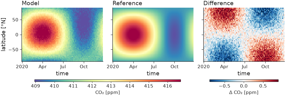
hovmoller() draws a field over time and one spatial coordinate; hovmoller_panels() lays out model, reference and difference with split colorbars, like cross_section_panels.

import nicefigs as nf
from nicefigs import data

nf.set_theme("paper")
h = data.hovmoller_field()
fig, axes = nf.hovmoller_panels(
    {"Model": h["value"], "Reference": h["reference"], "Difference": h["value"] - h["reference"]},
    h["times"],
    h["lats"],
    diff_fields={"Difference"},
    value_label="CO₂ [ppm]",
    diff_label="Δ CO₂ [ppm]",
)

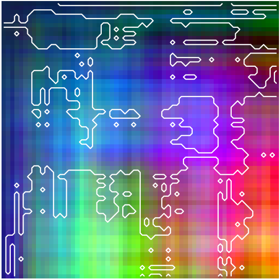
Composites of many channels

pca_rgb() projects an (H, W, C) field onto its first three principal components and returns a stretched (H, W, 3) image. With return_basis=True it also returns the projection and its colour limits; passing that basis to later calls keeps several patches on one colour scale. image(..., overlay_contour=mask) outlines a mask on top.

import numpy as np

import nicefigs as nf

nf.set_theme("paper")
rng = np.random.default_rng(0)
cube = rng.normal(size=(64, 64, 8)).cumsum(axis=0).cumsum(axis=1)
rgb, basis = nf.pca_rgb(cube, return_basis=True)
fig, ax = nf.subplots(width="single", aspect=1.0)
nf.image(rgb, overlay_contour=cube[..., 0] > np.median(cube[..., 0]), ax=ax)
print(rgb.shape, float(rgb.min()), float(rgb.max()))

(64, 64, 3) 0.0 1.0

Plotting eigen-spectra

spectrum() plots covariance eigenvalues λ_k against rank k on log–log axes, normalised to λ_k / Σλ by default. Pass one 1-D array, a list, or a {name: eigenvalues} dict to overlay several states; reference_alpha adds a k^-α power law through the first series' leading value:

import nicefigs as nf
from nicefigs import data

nf.set_theme("paper")
spectra = data.eigen_spectra()  # {"lead 6 h": λ, "lead 24 h": λ, "lead 72 h": λ}
fig, axes = nf.subplots(1, 2, width="full", aspect=0.42, layout="constrained")
nf.spectrum(spectra, ax=axes[0], reference_alpha=1.0)
nf.spectrum(spectra, ax=axes[1], cumulative=True, legend=False)

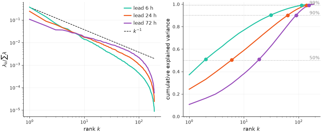
cumulative=True (right) plots the cumulative explained-variance fraction on a log rank axis, with one labelled dotted guide per threshold and a marker where each series first reaches it. Each spectrum is sorted descending and loses its non-finite, non-positive and round-off-sized (λ ≤ rtol · λ_max) eigenvalues, so the rank-deficient tail of a sample covariance does not distort the log axis; set rtol=0 to keep every positive eigenvalue.

Labelling axes with units and directions

axis_label() composes "Quantity [unit]" labels and prettifies the unit with prettify_unit(); a direction from DIRECTIONS appends an arrow. metric_label() looks a metric key up in METRIC_NAMES, and with direction=True its arrow in METRIC_DIRECTION.

import nicefigs as nf

print(nf.axis_label("flux", "gC m-2 d-1"))
print(nf.axis_label("skill", direction="higher_better"))
print(nf.metric_label("rmse", "mm", direction=True))

flux [gC m⁻² d⁻¹]
skill ↑
RMSE [mm] ↓

"target" adds no arrow; every helper that asks which way is better (scorecard, skill_gap, lines, pareto) takes the same three strings.