Gallery

Every example below is a full, runnable script under examples/ in the repository (examples/NN_*.py), each producing exactly one image in this gallery. All example data comes from nicefigs.data: deterministic, numpy-only synthetic fields, so the gallery, docs and tests draw the same figures from the same data.

Maps

01 — Global map

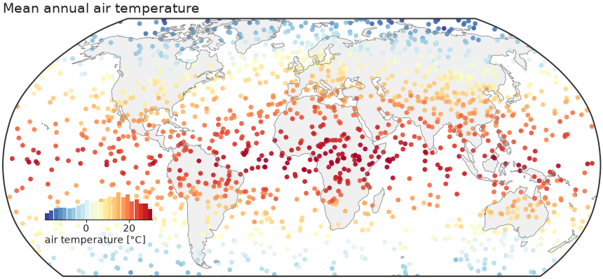
The house default: nicefigs.map scatters per-station values on a Robinson world map, crops Antarctica, and draws an inset histogram that doubles as the colorbar and shows the data distribution.

"""Global map — Robinson projection, Antarctica cropped, inset-histogram colorbar.

The house default: ``nicefigs.map`` scatters per-station values on a Robinson
world map, crops Antarctica, and draws an inset histogram that
doubles as the colorbar and shows the data distribution.
"""

import nicefigs as nf
from nicefigs import data


def make():
    nf.set_theme("paper")
    lon, lat, temp = data.global_points(field="temperature")
    fig, ax, _ = nf.map(
        lon,
        lat,
        temp,
        cmap="RdYlBu_r",
        colorbar_label="air temperature [°C]",
        title="Mean annual air temperature",
    )
    return fig


if __name__ == "__main__":
    import matplotlib

    matplotlib.use("Agg")
    nf.save(make(), "01_global_map", formats=("png", "pdf"))

02 — Anomaly map (binned)

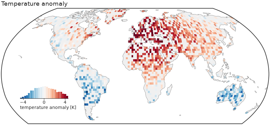
For dense fields, kind="binned" bin-averages onto a regular grid and masks the ocean. diverging=True picks a diverging colormap and symmetric limits about zero — the right default for anomalies.

"""Binned anomaly map — diverging colormap, ocean clipped, symmetric limits.

For dense fields, ``kind="binned"`` bin-averages onto a regular grid and masks
the ocean. ``diverging=True`` picks a diverging colormap and symmetric limits
about zero — the right default for anomalies.
"""

import nicefigs as nf
from nicefigs import data


def make():
    nf.set_theme("paper")
    lon, lat, anom = data.global_points(n=9000, field="anomaly")
    fig, ax, _ = nf.map(
        lon,
        lat,
        anom,
        kind="binned",
        diverging=True,
        colorbar_label="temperature anomaly [K]",
        title="Temperature anomaly",
        bin_deg=2.5,
    )
    return fig


if __name__ == "__main__":
    import matplotlib

    matplotlib.use("Agg")
    nf.save(make(), "02_anomaly_map", formats=("png", "pdf"))

03 — Regional map

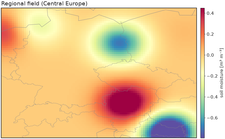
A bounded extent on a Plate Carrée axes with a slim colorbar instead of the inset histogram.

"""Regional map — a bounded extent on a Plate Carrée axes with a slim colorbar."""

import nicefigs as nf
from nicefigs import data


def make():
    nf.set_theme("paper")
    lon2d, lat2d, z = data.regional_grid(extent=(5, 20, 45, 55), res=0.08)
    fig, ax, m = nf.map(
        lon2d.ravel(),
        lat2d.ravel(),
        z.ravel(),
        extent=(5, 20, 45, 55),
        projection="platecarree",
        kind="binned",
        bin_deg=0.15,
        cmap="Spectral_r",
        inset_hist=False,
        cbar=True,
        colorbar_label="soil moisture [m³ m⁻³]",
        borders=True,
        title="Regional field (Central Europe)",
    )
    return fig


if __name__ == "__main__":
    import matplotlib

    matplotlib.use("Agg")
    nf.save(make(), "03_regional_map", formats=("png", "pdf"))

04 — Shared colorbar across subplots

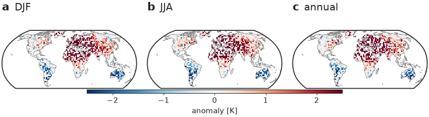
One colorbar serves a whole row of maps (no repetition), and the with nf.style(...) context manager restyles otherwise-plain matplotlib code — drop it on top of anything.

"""Shared colorbar across subplots + the ``with nf.style(...)`` context manager.

One colorbar serves a whole row of maps (no repetition), and the context manager
restyles otherwise-plain matplotlib code — drop it on top of anything.
"""

import nicefigs as nf
from nicefigs import data


def make():
    import cartopy.crs as ccrs

    # The context manager applies the house style just for this block.
    with nf.style("paper"):
        fig, axes = nf.subplots(
            1,
            3,
            width="full",
            panel_aspect=0.62,
            subplot_kw={"projection": ccrs.Robinson()},
            wspace=0.08,
        )
        seasons = ["DJF", "JJA", "annual"]
        m = None
        for si, ax in enumerate(axes):
            lon, lat, v = data.global_points(n=6000, field="anomaly", seed=si + 1)
            nf.draw_background(ax, ccrs)
            ax.set_extent(nf.maps.ANTARCTICA_CUTOFF_EXTENT, crs=ccrs.PlateCarree())
            _, m = nf.binned_map(
                lon,
                lat,
                v,
                ccrs=ccrs,
                cmap="RdBu_r",
                vmin=-2.5,
                vmax=2.5,
                bin_deg=3.0,
                clip_ocean=True,
                ax=ax,
            )
        # one bar spans all three panels
        nf.colorbar(m, list(axes), label="anomaly [K]", location="bottom", thickness=0.03, shrink=0.6)
        # combined label + short title (no separate set_title → no collision)
        nf.label_panels(axes, titles=seasons)
    return fig


if __name__ == "__main__":
    import matplotlib

    matplotlib.use("Agg")
    nf.save(make(), "04_shared_colorbar", formats=("png", "pdf"))

05 — Ternary map

A global/regional map whose points are coloured by a 3-part composition, with a triangular legend inset that decodes the colours.

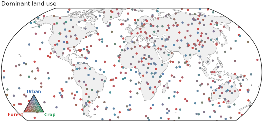
"""Ternary map — locations coloured by a 3-part composition, with a legend inset."""

import nicefigs as nf
from nicefigs import data


def make():
    nf.set_theme("paper")
    comp, _ = data.ternary_points(n=1400)
    lon, lat, _ = data.global_points(n=1400)
    n = min(len(comp), len(lon))
    fig, ax = nf.ternary_map(
        lon[:n],
        lat[:n],
        comp[:n],
        labels=("Forest", "Crop", "Urban"),
        size=7,
        title="Dominant land use",
    )
    return fig


if __name__ == "__main__":
    import matplotlib

    matplotlib.use("Agg")
    nf.save(make(), "05_ternary_map", formats=("png", "pdf"))

06 — Bivariate colormap

nicefigs.colormaps2d encodes two continuous variables in one colour via a 2D palette — here bivariate_cmap (a 4-corner bilinear blend), decoded by a square bivariate_legend inset. hsv_cmap and flat_cmap (a constant-lightness CIE-Lab wheel) are drop-in alternatives with their own hsv_legend/flat_legend.

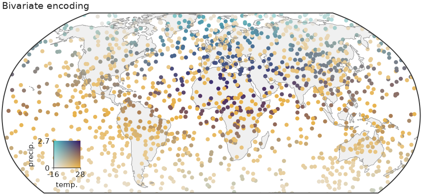
"""Bivariate (2D) colormap — encode two variables at once, with a square legend.

A global scatter coloured by a 2D palette (one variable → x-axis of the colour
square, the other → y-axis), with the key drawn as an inset.
"""

import nicefigs as nf
from nicefigs import data
from nicefigs.colormaps2d import normalize01


def make():
    nf.set_theme("paper")
    lon, lat, temp = data.global_points(field="temperature")
    _, _, precip = data.global_points(field="sparse")
    n = min(len(temp), len(precip))
    lon, lat, temp, precip = lon[:n], lat[:n], temp[:n], precip[:n]

    tx, trange = normalize01(temp)
    py, prange = normalize01(precip)
    colors = nf.bivariate_cmap(tx, py)

    # Build the map ourselves so the points carry the 2D colours directly.
    fig = nf.figure(width="full", aspect=0.52)
    ax, ccrs = nf.make_map_axes(fig, 111, projection="robinson")
    nf.draw_background(ax, ccrs)
    ax.set_extent(nf.maps.ANTARCTICA_CUTOFF_EXTENT, crs=ccrs.PlateCarree())
    ax.scatter(lon, lat, c=colors, s=9, linewidths=0, transform=ccrs.PlateCarree(), rasterized=True)
    nf.clean_title(ax, "Bivariate encoding")

    iax = ax.inset_axes([0.08, 0.14, 0.15, 0.15])
    iax.patch.set_alpha(0.0)
    nf.bivariate_legend(iax, x_label="temp.", y_label="precip.", x_range=trange, y_range=prange)
    return fig


if __name__ == "__main__":
    import matplotlib

    matplotlib.use("Agg")
    nf.save(make(), "06_bivariate", formats=("png", "pdf"))

Images & colormaps

07 — Image grid

Several heatmaps on a shared colour scale with one colorbar for the whole grid.

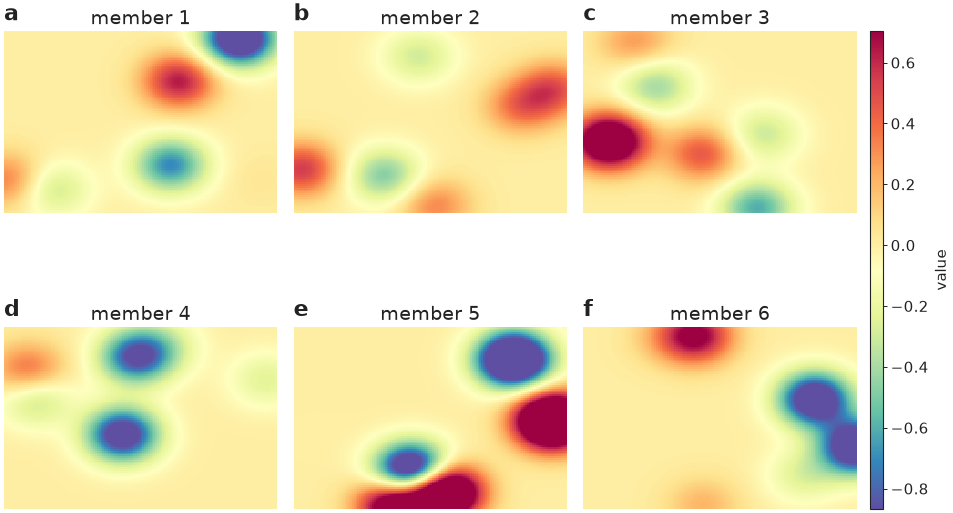
"""Image grid — several heatmaps on a shared colour scale with one colorbar."""

import nicefigs as nf
from nicefigs import data


def make():
    nf.set_theme("paper")
    imgs = [data.regional_grid(seed=i)[2] for i in range(6)]
    fig, axes = nf.image_grid(
        imgs,
        nrows=2,
        ncols=3,
        cmap="Spectral_r",
        colorbar_label="value",
        titles=[f"member {i + 1}" for i in range(6)],
    )
    nf.label_panels(axes)
    return fig


if __name__ == "__main__":
    import matplotlib

    matplotlib.use("Agg")
    nf.save(make(), "07_image_grid", formats=("png", "pdf"))

08 — RGB imagery & land cover

Natural-colour imagery next to a categorical land-cover raster with a geospecific palette and matching legend.

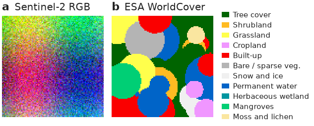
"""RGB imagery + categorical land cover — a geospecific palette with a legend."""

import nicefigs as nf
from nicefigs import data


def make():
    nf.set_theme("paper")
    fig, axes = nf.subplots(1, 2, width="half", panel_aspect=1.0, wspace=0.08)
    nf.image(data.rgb_patch(), rgb=True, stretch=True, ax=axes[0])

    lc = nf.categorical("esa_worldcover")
    nf.image(lc.to_rgb(data.landcover_patch()), rgb=True, ax=axes[1])
    axes[1].legend(
        handles=lc.legend_handles(),
        loc="center left",
        bbox_to_anchor=(1.02, 0.5),
        fontsize=nf.get_theme().fs_annot,
        frameon=False,
        handlelength=1.0,
        labelspacing=0.35,
    )
    # combined label + title (top-left) avoids clashing with a centred title
    nf.label_panels(axes, titles=["Sentinel-2 RGB", "ESA WorldCover"])
    return fig


if __name__ == "__main__":
    import matplotlib

    matplotlib.use("Agg")
    nf.save(make(), "08_landcover_rgb", formats=("png", "pdf"))

09 — Annotated heatmap

A labelled heatmap with row/column labels, cell annotations, and a tight colorbar.

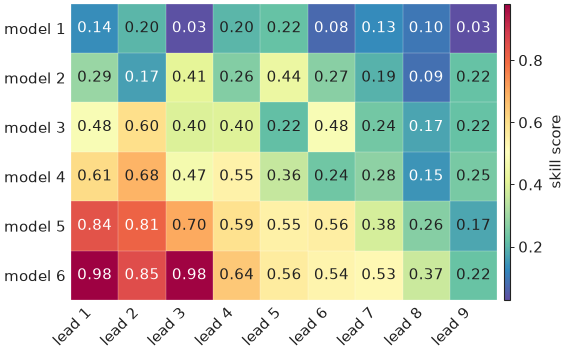
"""Annotated heatmap — labelled rows/columns with a tight colorbar."""

import nicefigs as nf
from nicefigs import data


def make():
    nf.set_theme("paper")
    fig, ax = nf.subplots(width="half", aspect=0.7)
    _, m = nf.heatmap(
        data.heatmap_matrix(shape=(6, 9)),
        row_labels=[f"model {i + 1}" for i in range(6)],
        col_labels=[f"lead {i + 1}" for i in range(9)],
        cmap="Spectral_r",
        annotate=True,
        ax=ax,
    )
    nf.colorbar(m, ax, label="skill score")
    return fig


if __name__ == "__main__":
    import matplotlib

    matplotlib.use("Agg")
    nf.save(make(), "09_heatmap", formats=("png", "pdf"))

10 — Elevation colormap

A geoscience-specific colormap: a hypsometric elevation ramp with a sea-level break, built by elevation_cmap.

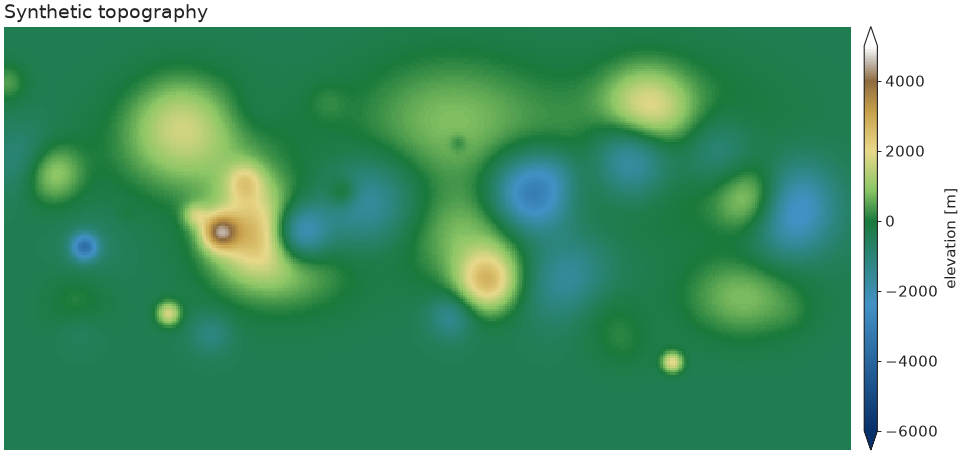
"""Geoscience colormap — hypsometric elevation ramp with a sea-level break."""

import nicefigs as nf
from nicefigs import data


def make():
    nf.set_theme("paper")
    z = data.elevation_field()
    cmap, norm = nf.elevation_cmap(vmin=-6000, vmax=5000)
    fig, ax = nf.subplots(width="full", aspect=0.5)
    _, m = nf.image(z, cmap=cmap, norm=norm, extent=(-180, 180, -90, 90), ax=ax)
    nf.colorbar(m, ax, label="elevation [m]", extend="both")
    nf.clean_title(ax, "Synthetic topography")
    return fig


if __name__ == "__main__":
    import matplotlib

    matplotlib.use("Agg")
    nf.save(make(), "10_elevation", formats=("png", "pdf"))

11 — Ternary scatter

A composition (a, b, c) with a + b + c = 1 — here soil texture — encoded as colour by blending three corner colours barycentrically, scattered inside a triangular frame.

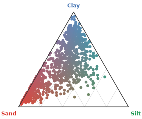
"""Ternary scatter — soil texture compositions coloured by their mixture."""

import nicefigs as nf
from nicefigs import data


def make():
    nf.set_theme("paper")
    comp, _ = data.ternary_points(n=900)
    ax, _ = nf.ternary_scatter(comp, labels=("Sand", "Silt", "Clay"), size=12)
    return ax.figure


if __name__ == "__main__":
    import matplotlib

    matplotlib.use("Agg")
    nf.save(make(), "11_ternary", formats=("png", "pdf"))

12 — Artist-inspired palettes

Painterly categorical palettes ported from MetBrewer and MoMAColors (artist_palette), plus two bespoke categorical bases extracted from David Hockney's A Bigger Grand Canyon (1998): HOCKNEY_CANYON ("hockney"), wired into cmap("hockney_canyon") as a continuous colormap (artist_cmap); and NICE ("nice") — a bright teal leading the same Hockney family — which is the house default categorical cycle, used by every theme and by qualitative() whenever no palette is given.

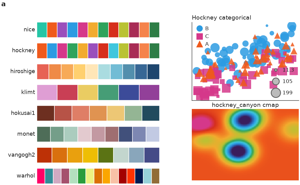
"""Artist-inspired palettes — painterly categorical schemes + the Hockney base.

Swatches for a selection of MetBrewer / MoMAColors palettes and the bespoke
David-Hockney *A Bigger Grand Canyon* categorical base, plus two demos that use
it: a grouped scatter and a field coloured by the ``hockney_canyon`` colormap.
"""

import matplotlib.pyplot as plt

import nicefigs as nf
from nicefigs import data

SHOWCASE = ["nice", "hockney", "hiroshige", "klimt", "hokusai1", "monet", "vangogh2", "warhol"]


def _swatch(ax, name):
    cols = nf.artist_palette(name)
    for i, c in enumerate(cols):
        ax.add_patch(plt.Rectangle((i, 0), 1, 1, facecolor=c, edgecolor="white", linewidth=0.6))
    ax.set_xlim(0, max(len(cols), 1))
    ax.set_ylim(0, 1)
    ax.set_xticks([])
    ax.set_yticks([])
    for sp in ax.spines.values():
        sp.set_visible(False)
    ax.set_ylabel(name, rotation=0, ha="right", va="center", fontsize=nf.get_theme().fs_axis_label)


def make():
    nf.set_theme("paper")
    fig = nf.figure(width="full", aspect=0.62)
    gs = fig.add_gridspec(len(SHOWCASE), 2, width_ratios=[1.15, 1.0], wspace=0.28, hspace=0.35)

    # (a) palette swatches
    for i, name in enumerate(SHOWCASE):
        ax = fig.add_subplot(gs[i, 0])
        _swatch(ax, name)
    fig.text(0.02, 0.98, "a", fontsize=nf.get_theme().fs_panel_label, fontweight="bold", va="top")

    # (b) Hockney categorical scatter
    ax_sc = fig.add_subplot(gs[: len(SHOWCASE) // 2, 1])
    d = data.scatter_bubbles(n=150)
    nf.scatter(
        d["x"],
        d["y"],
        group=d["group"],
        group_colors=dict(zip(["A", "B", "C"], nf.qualitative(3, "hockney"))),
        size=d["size"],
        size_label="",
        legend=True,
        ax=ax_sc,
    )
    nf.clean_title(ax_sc, "Hockney categorical")
    ax_sc.set_xticks([])
    ax_sc.set_yticks([])

    # (c) Hockney continuous colormap on a field
    ax_im = fig.add_subplot(gs[len(SHOWCASE) // 2 :, 1])
    _, _, z = data.regional_grid(seed=3)
    nf.image(z, cmap="hockney_canyon", robust=True, title="hockney_canyon cmap", ax=ax_im)

    return fig


if __name__ == "__main__":
    import matplotlib

    matplotlib.use("Agg")
    nf.save(make(), "12_artist_palettes", formats=("svg", "png"))

Composition

The same barycentric colour encoding — nicefigs.ternary.color — underlies every ternary helper, which is what lets it drop onto different plot kinds without change: example 11 applies it to a scatter inside a triangular frame (ternary_scatter), while example 05 applies the identical encoding to points on a global map (ternary_map), reusing ternary_legend as the inset in both cases. This is the composability nicefigs is built around: small helpers that all take an existing ax, so they combine freely instead of each owning a whole figure. See the Composite figure below for the same idea applied across map, timeseries, and agreement panels in one GridSpec.

Relational & distributions

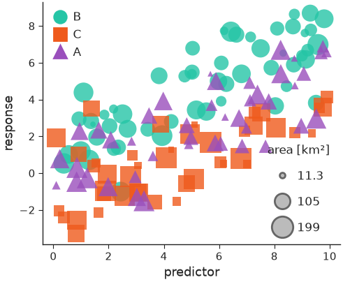
13 — Multi-encoding scatter

Marker shape (a categorical group), size (a continuous variable), and colour map onto up to three extra variables, with a compact legend for each.

"""Scatter with three encodings — marker shape (group), size, and colour."""

import nicefigs as nf
from nicefigs import data


def make():
    nf.set_theme("paper")
    d = data.scatter_bubbles(n=140)
    fig, ax = nf.subplots(width="half", aspect=0.82)
    nf.scatter(
        d["x"],
        d["y"],
        group=d["group"],
        size=d["size"],
        size_label="area [km²]",
        alpha=0.8,
        ax=ax,
    )
    nf.set_labels(ax, "predictor", "response")
    return fig


if __name__ == "__main__":
    import matplotlib

    matplotlib.use("Agg")
    nf.save(make(), "13_scatter", formats=("png", "pdf"))

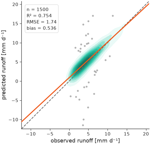
14 — Agreement plot

The house predicted-vs-observed plot: a KDE density of the bulk of the cloud, a dashed 1:1 line, outliers as faint scatter, a solid regression line, and a compact metrics box (n, R², RMSE, bias).

"""Agreement plot — KDE density, 1:1 line, outlier scatter, regression, metrics."""

import nicefigs as nf
from nicefigs import data


def make():
    nf.set_theme("paper")
    obs, pred = data.xy_agreement(r=0.92)
    ax, stats = nf.agreement(
        obs,
        pred,
        xlabel="observed runoff",
        ylabel="predicted runoff",
        units="mm d⁻¹",
    )
    return ax.figure


if __name__ == "__main__":
    import matplotlib

    matplotlib.use("Agg")
    nf.save(make(), "14_agreement", formats=("png", "pdf"))

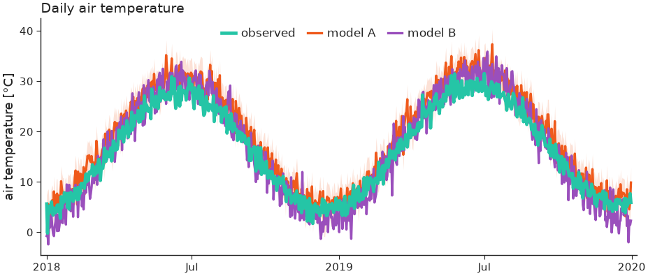
15 — Timeseries

Observations vs. models with an uncertainty band and a date axis that adapts its ticks/format to the observed time span.

"""Timeseries — observations vs models with an uncertainty band and date axis."""

import nicefigs as nf
from nicefigs import data


def make():
    nf.set_theme("paper")
    dates, series = data.timeseries(n_days=730)
    # a simple uncertainty band around model A
    a = series["model A"]
    bands = {"model A": (a - 3, a + 3)}
    ax = nf.timeseries(
        dates,
        series,
        bands=bands,
        highlight="observed",
        ylabel="air temperature",
        yunits="degC",
        title="Daily air temperature",
    )
    return ax.figure


if __name__ == "__main__":
    import matplotlib

    matplotlib.use("Agg")
    nf.save(make(), "15_timeseries", formats=("png", "pdf"))

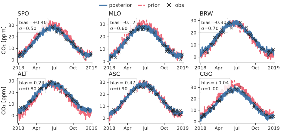
16 — Faceted station timeseries

Small-multiples of per-station model curtains with a sparse observation overlay, built from nicefigs.facet (one call per panel, consistent physical sizing) plus timeseries's obs= overlay, per-series styles, and a per-panel annotation.

"""Faceted station timeseries — model curtains + sparse observations per station.

Uses ``nicefigs.facet`` for the small-multiples grid and ``timeseries``'s
observation overlay + per-panel annotation.
"""

import numpy as np

import nicefigs as nf
from nicefigs import data


def make():
    nf.set_theme("paper")
    stations = ["SPO", "MLO", "BRW", "ALT", "ASC", "CGO"]

    def draw(ax, station, i):
        dates, series = data.timeseries(n_days=365, seed=i + 1, series=["posterior", "prior"])
        rng = np.random.default_rng(i)
        idx = np.sort(rng.choice(365, 36, replace=False))
        obs = ([dates[k] for k in idx], series["posterior"][idx] + rng.normal(0, 1, 36))
        nf.timeseries(
            dates,
            series,
            ax=ax,
            obs=obs,
            obs_label="obs",
            styles={"prior": "--", "posterior": "-"},
            highlight="posterior",
            colors={"posterior": "#4477AA", "prior": "#EE6677"},
            annotation=f"bias={rng.normal(0, 0.4):+.2f}\nσ={0.5 + 0.1 * i:.2f}",
            ylabel="CO₂" if i % 3 == 0 else "",
            yunits="ppm",
            legend=False,
        )

    fig, axes = nf.facet(stations, draw, ncols=3, panel_aspect=0.62, titles=stations)
    # one shared legend for the whole figure
    import matplotlib.lines as ml

    handles = [
        ml.Line2D([], [], color="#4477AA", label="posterior"),
        ml.Line2D([], [], color="#EE6677", ls="--", label="prior"),
        ml.Line2D(
            [], [], color="#222222", marker="x", ls="None", markersize=4, markeredgewidth=0.8, label="obs"
        ),
    ]
    fig.legend(
        handles=handles,
        loc="upper center",
        bbox_to_anchor=(0.5, 1.02),
        ncol=3,
        fontsize=nf.get_theme().fs_legend,
        frameon=False,
    )
    return fig


if __name__ == "__main__":
    import matplotlib

    matplotlib.use("Agg")
    nf.save(make(), "16_station_timeseries", formats=("png", "pdf"))

32 — Eigen-spectra

nicefigs.spectrum plots covariance eigenvalue spectra against rank on log–log axes (left, with a k^-1 reference power law) or as cumulative explained variance with markers where each series reaches 50, 90 and 99 % (right). Numerically zero tails are dropped.

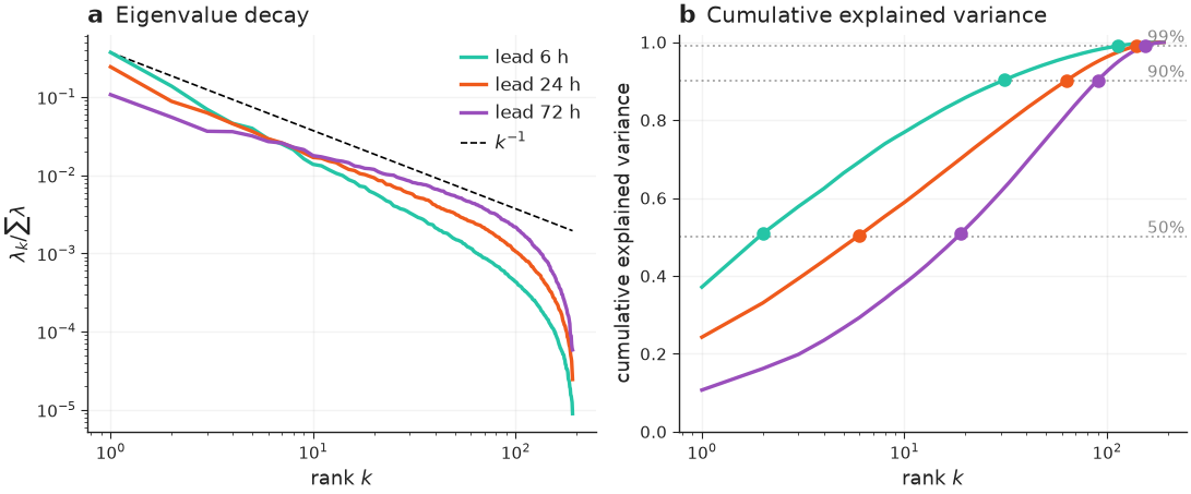
"""Eigen-spectra — eigenvalue decay and cumulative explained variance, side by side."""

import nicefigs as nf
from nicefigs import data


def make():
    nf.set_theme("paper")
    spectra = data.eigen_spectra()
    fig, (ax1, ax2) = nf.subplots(1, 2, width="full", aspect=0.42, layout="constrained")
    nf.spectrum(spectra, ax=ax1, reference_alpha=1.0, title="Eigenvalue decay")
    nf.spectrum(spectra, ax=ax2, cumulative=True, legend=False, title="Cumulative explained variance")
    nf.label_panels([ax1, ax2], use_ax_title=True)
    return fig


if __name__ == "__main__":
    import matplotlib

    matplotlib.use("Agg")
    nf.save(make(), "32_spectrum", formats=("png", "pdf"))

Comparison & ranking

17 — Model comparison

One panel per metric, a violin per model, dodged by an optional group (e.g. timescale), with a single shared legend.

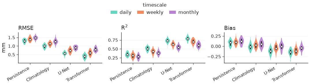
"""Model comparison — one panel per metric, a violin per model, split by timescale."""

import nicefigs as nf
from nicefigs import data


def make():
    nf.set_theme("paper")
    scores = data.model_scores()
    fig, axes = nf.model_comparison(
        scores,
        group_label="timescale",
        kind="violin",
        metric_units={"RMSE": "mm"},
    )
    return fig


if __name__ == "__main__":
    import matplotlib

    matplotlib.use("Agg")
    nf.save(make(), "17_model_comparison", formats=("png", "pdf"))

18 — Pareto frontier

nicefigs.pareto scatters a trade-off (here speed vs. skill) with the non-dominated frontier drawn per group, arrows from xdirection/ydirection on the axis labels showing which way is better, and labelled baselines as reference lines.

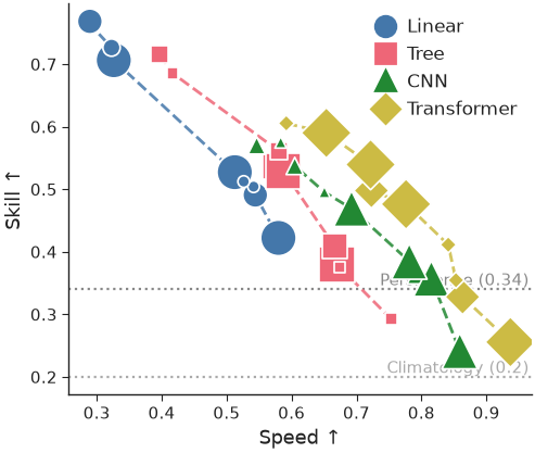
"""Pareto plot — a speed vs skill trade-off, one frontier per model family."""

import nicefigs as nf
from nicefigs import data


def make():
    nf.set_theme("paper")
    d = data.pareto_tradeoff()
    ax, _ = nf.pareto(
        d["x"],
        d["y"],
        group=d["group"],
        size=d["size"],
        group_colors={
            "Linear": "#4477AA",
            "Tree": "#EE6677",
            "CNN": "#228833",
            "Transformer": "#CCBB44",
        },
        frontier_per_group=True,
        xdirection="higher_better",
        ydirection="higher_better",
        xlabel="Speed",
        ylabel="Skill",
        baselines={"Persistence": 0.34, "Climatology": 0.20},
    )
    return ax.figure


if __name__ == "__main__":
    import matplotlib

    matplotlib.use("Agg")
    nf.save(make(), "18_pareto", formats=("png", "pdf"))

19 — Caterpillar / forest plot

nicefigs.caterpillar ranks per-item values ± error (here per-site bias ± σ), with an optional baseline series offset alongside each item, a reference line at the null, and a headline summary annotation.

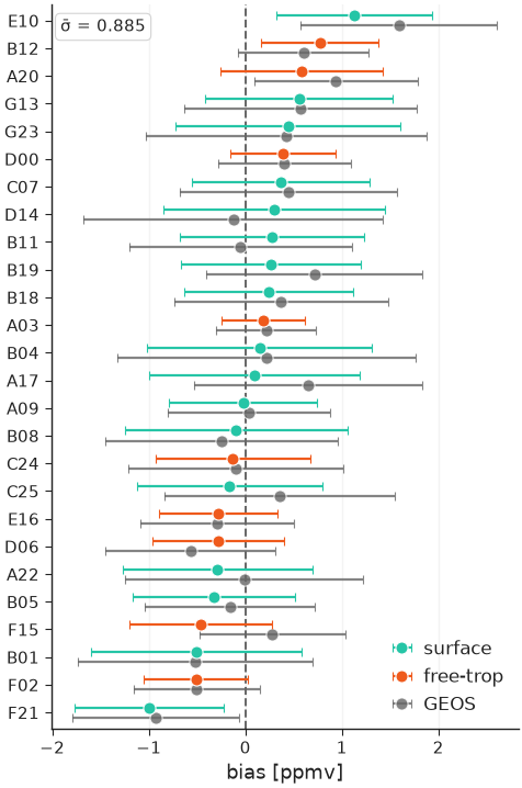
"""Caterpillar / forest plot — per-site bias ± σ, ranked, with a baseline model."""

import numpy as np

import nicefigs as nf
from nicefigs import data


def make():
    nf.set_theme("paper")
    s = data.site_metrics(n_sites=26)
    ax = nf.caterpillar(
        s["labels"],
        s["bias"],
        err=s["std"],
        groups=s["layer"],
        baseline=s["baseline"],
        baseline_label="GEOS",
        value_label="bias",
        value_units="ppmv",
        summary=("σ̄", float(np.sqrt(np.mean(s["std"] ** 2)))),
        ref_line=0.0,
    )
    return ax.figure


if __name__ == "__main__":
    import matplotlib

    matplotlib.use("Agg")
    nf.save(make(), "19_caterpillar", formats=("png", "pdf"))

20 — Scorecard

nicefigs.scorecard renders a model×metric table as coloured cells — normalised independently per column and respecting each metric's direction (lower/higher better) — with the best model per metric outlined.

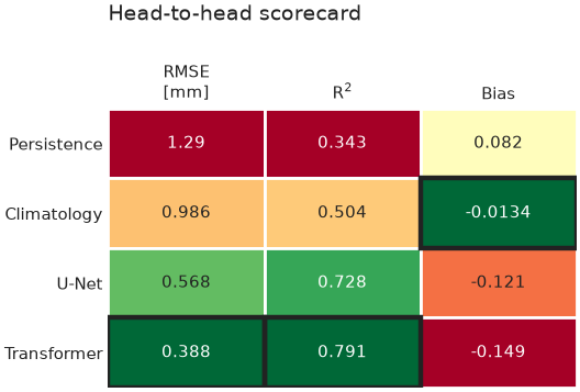
"""Scorecard — a model×metric table coloured per column by how good each value is."""

import numpy as np

import nicefigs as nf
from nicefigs import data


def make():
    nf.set_theme("paper")
    ms = data.model_scores()
    models, metrics = ms["models"], ms["metrics"]
    vals = np.array([[np.mean(ms["scores"][m][mdl]["daily"]) for m in metrics] for mdl in models])
    ax = nf.scorecard(
        vals,
        row_labels=models,
        col_labels=metrics,
        direction={"RMSE": "lower_better", "Bias": "target", "R$^2$": "higher_better"},
        col_units={"RMSE": "mm"},
        title="Head-to-head scorecard",
    )
    return ax.figure


if __name__ == "__main__":
    import matplotlib

    matplotlib.use("Agg")
    nf.save(make(), "20_scorecard", formats=("png", "pdf"))

21 — Grouped & stacked bars

nicefigs.grouped_bars dodges one bar per (category, series); nicefigs.stacked_bars stacks series within each category (normalize=True for fractions) — both take a plain ax so they drop into any layout.

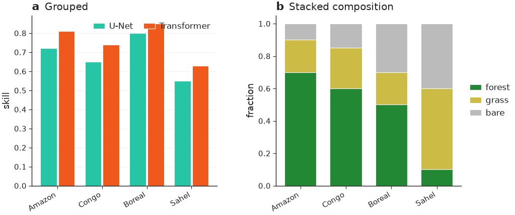
"""Grouped and stacked bars — models × metric, and land-cover composition."""

import nicefigs as nf


def make():
    nf.set_theme("paper")
    fig, axes = nf.subplots(1, 2, width="full", panel_aspect=0.8, wspace=0.32)

    regions = ["Amazon", "Congo", "Boreal", "Sahel"]
    nf.grouped_bars(
        regions,
        {"U-Net": [0.72, 0.65, 0.80, 0.55], "Transformer": [0.81, 0.74, 0.85, 0.63]},
        value_label="skill",
        rotation=30,
        ax=axes[0],
    )
    nf.stacked_bars(
        regions,
        {"forest": [0.7, 0.6, 0.5, 0.1], "grass": [0.2, 0.25, 0.2, 0.5], "bare": [0.1, 0.15, 0.3, 0.4]},
        normalize=True,
        rotation=30,
        colors={"forest": "#228833", "grass": "#CCBB44", "bare": "#BBBBBB"},
        ax=axes[1],
    )
    nf.label_panels(axes, titles=["Grouped", "Stacked composition"])
    return fig


if __name__ == "__main__":
    import matplotlib

    matplotlib.use("Agg")
    nf.save(make(), "21_bars", formats=("png", "pdf"))

30 — Scorecard, diverging

nicefigs.scorecard's opt-in kwargs for a WeatherBench2-style skill scorecard: an explicit diverging norm (here scorecard_diverging_cmap) colours cells by their actual percent-difference value anchored at zero instead of per-column goodness ranking; col_groups clusters columns with a gap and a group title; square=True forces square cells; colorbar=True draws a horizontal bar with the colormap's extend triangles.

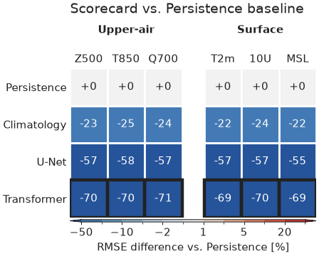
"""Scorecard with the WeatherBench2-inspired diverging colormap, grouped columns, and a colour bar."""

import numpy as np

import nicefigs as nf
from nicefigs import data


def make():
    nf.set_theme("paper")
    models = ["Persistence", "Climatology", "U-Net", "Transformer"]
    variables = ["Z500", "T850", "Q700", "T2m", "10U", "MSL"]
    groups = ["Upper-air"] * 3 + ["Surface"] * 3

    # Percent RMSE difference of each model vs. the Persistence baseline, per
    # variable — the shape a WeatherBench2-style skill scorecard compares.
    pct_diff = np.zeros((len(models), len(variables)))
    for j in range(len(variables)):
        ms = data.model_scores(seed=100 + j, models=models, metrics=["RMSE"], timescales=["daily"])
        rmse = np.array([np.mean(ms["scores"]["RMSE"][m]["daily"]) for m in models])
        pct_diff[:, j] = 100.0 * (rmse - rmse[0]) / rmse[0]

    cmap, norm = nf.scorecard_diverging_cmap()
    ax = nf.scorecard(
        pct_diff,
        row_labels=models,
        col_labels=variables,
        cmap=cmap,
        norm=norm,
        direction=dict.fromkeys(variables, "lower_better"),
        col_groups=groups,
        square=True,
        cell_format="{:+.0f}",
        colorbar=True,
        colorbar_label="RMSE difference vs. Persistence [%]",
        title="Scorecard vs. Persistence baseline",
    )
    return ax.figure


if __name__ == "__main__":
    import matplotlib

    matplotlib.use("Agg")
    nf.save(make(), "30_scorecard_diverging", formats=("png", "pdf"))

Vertical structure

22 — Cross-section / curtain

nicefigs.cross_section_panels lays out several latitude×pressure curtains (cross_section per panel) with shared value/difference colorbars — diff_fields routes named fields onto a symmetric, diverging scale, and log_y log-scales the vertical (pressure) axis.

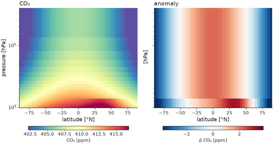
"""Cross-section / curtain — latitude × pressure, value and anomaly panels."""

import nicefigs as nf
from nicefigs import data


def make():
    nf.set_theme("paper")
    cs = data.cross_section_field()
    val = cs["value"]
    anom = val - val.mean(axis=0, keepdims=True)
    fig, axes = nf.cross_section_panels(
        {"CO₂": val, "anomaly": anom},
        cs["lats"],
        cs["levels"],
        diff_fields={"anomaly"},
        value_label="CO₂ [ppm]",
        diff_label="Δ CO₂ [ppm]",
        log_y=True,
    )
    return fig


if __name__ == "__main__":
    import matplotlib

    matplotlib.use("Agg")
    nf.save(make(), "22_cross_section", formats=("png", "pdf"))

Composite & animation

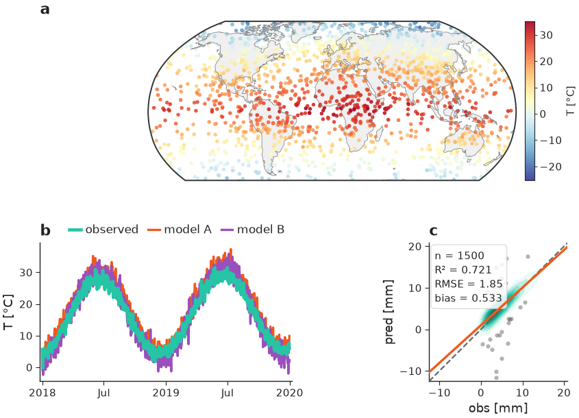
23 — Composite publication figure

Shows the pieces composing: a GridSpec from nicefigs.grid (a projected map panel plus two analysis panels), a colorbar hugging the map, and (a) (b) (c) panel labels — all at a single physical width so fonts stay consistent across every panel, whether it's a map, a timeseries, or a scatter plot.

"""Composite publication figure — maps, timeseries and agreement in one layout.

Shows the pieces composing: a GridSpec from ``nicefigs.grid`` (a projected map
panel plus two analysis panels), a colorbar hugging the map, and ``(a) (b) (c)``
panel labels — all at a single physical width so fonts stay consistent.
"""

import nicefigs as nf
from nicefigs import data


def make():
    nf.set_theme("paper")
    fig = nf.figure(width="full", aspect=0.62)
    gs = fig.add_gridspec(2, 2, height_ratios=[1.15, 1.0], hspace=0.42, wspace=0.32)

    # (a) global map spanning the top row
    ax_map, ccrs = nf.make_map_axes(fig, gs[0, :], projection="robinson")
    lon, lat, temp = data.global_points(field="temperature")
    _, m = nf.scatter_map(lon, lat, temp, ccrs=ccrs, cmap="RdYlBu_r", size=4, ax=ax_map)
    nf.draw_background(ax_map, ccrs)
    ax_map.set_extent(nf.maps.ANTARCTICA_CUTOFF_EXTENT, crs=ccrs.PlateCarree())
    nf.colorbar(m, ax_map, label="T [°C]")

    # (b) timeseries
    ax_ts = fig.add_subplot(gs[1, 0])
    dates, series = data.timeseries(n_days=730)
    nf.timeseries(dates, series, ax=ax_ts, highlight="observed", ylabel="T", yunits="degC", legend=False)
    ax_ts.legend(
        loc="lower right",
        bbox_to_anchor=(1.0, 1.0),
        ncol=3,
        frameon=False,
        borderaxespad=0.2,
        handlelength=1.0,
        handletextpad=0.4,
        columnspacing=0.8,
    )

    # (c) agreement
    ax_ag = fig.add_subplot(gs[1, 1])
    obs, pred = data.xy_agreement()
    nf.agreement(obs, pred, ax=ax_ag, xlabel="obs", ylabel="pred", units="mm")

    nf.label_panels([ax_map, ax_ts, ax_ag])
    return fig


if __name__ == "__main__":
    import matplotlib

    matplotlib.use("Agg")
    nf.save(make(), "23_composite_figure", formats=("png", "pdf"))

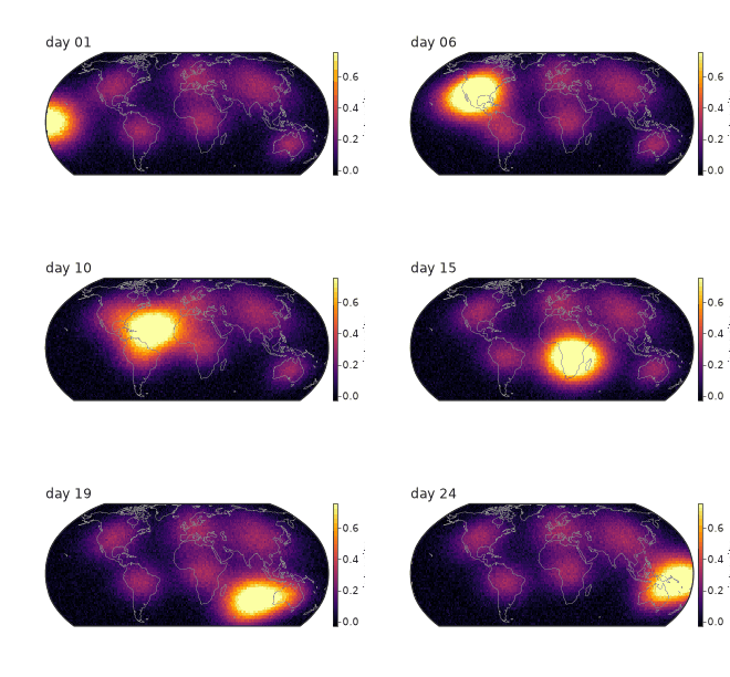
24 — Map animation

A drifting field animated over a fixed colour scale (computed once across all frames so colours are comparable frame-to-frame), saved to GIF.

"""Map animation — a drifting field with a fixed colour scale, saved to GIF."""

import nicefigs as nf
from nicefigs import data


def make(path="24_animation.gif"):
    nf.set_theme("paper")
    lon, lat, frames = data.map_timeseries_cube(n_frames=24)
    fig, _, anim = nf.animate_maps(
        lon,
        lat,
        frames,
        cmap="inferno",
        titles=[f"day {i + 1:02d}" for i in range(len(frames))],
        colorbar_label="intensity",
        fps=8,
    )
    out = nf.save_animation(anim, path, fps=8)
    return out


if __name__ == "__main__":
    import matplotlib

    matplotlib.use("Agg")
    print("wrote", make())

Model evaluation & time–space

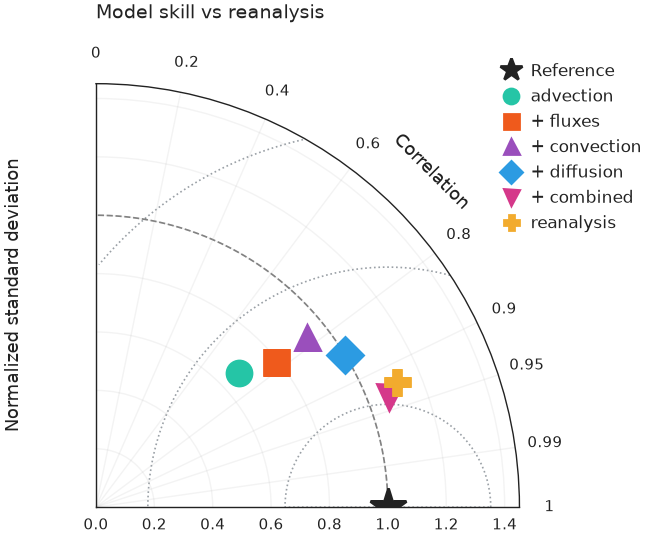
25 — Taylor diagram

nicefigs.taylor summarises correlation, standard deviation and centred RMS difference against a reference in one polar plot — the standard one-glance model-evaluation chart. Pass one entry per model with a correlation and either an absolute std or a normalised std_ratio.

"""Taylor diagram — correlation, standard deviation and centred RMS at a glance."""

import nicefigs as nf
from nicefigs import data


def make():
    nf.set_theme("paper")
    ax = nf.taylor(data.taylor_stats(), title="Model skill vs reanalysis")
    return ax.figure


if __name__ == "__main__":
    import matplotlib

    matplotlib.use("Agg")
    nf.save(make(), "25_taylor", formats=("png", "pdf"))

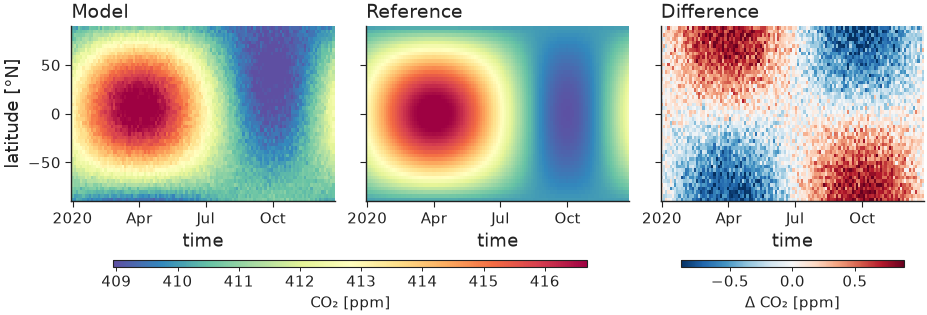
26 — Hovmöller diagram

nicefigs.hovmoller plots a field over one spatial coordinate and time; nicefigs.hovmoller_panels lays out model, reference and their difference with shared value / difference colorbars. The time axis accepts numbers or datetime objects.

"""Hovmöller diagram — a latitude × time field, with model / reference / difference."""

import nicefigs as nf
from nicefigs import data


def make():
    nf.set_theme("paper")
    h = data.hovmoller_field()
    diff = h["value"] - h["reference"]
    fig, _ = nf.hovmoller_panels(
        {"Model": h["value"], "Reference": h["reference"], "Difference": diff},
        h["times"],
        h["lats"],
        diff_fields={"Difference"},
        value_label="CO₂ [ppm]",
        diff_label="Δ CO₂ [ppm]",
    )
    return fig


if __name__ == "__main__":
    import matplotlib

    matplotlib.use("Agg")
    nf.save(make(), "26_hovmoller", formats=("png", "pdf"))

27 — Vertical profile

nicefigs.profile is the 1-D companion to cross_section: several profiles (value vs level/pressure) with an inverted, optionally log-scaled vertical axis and dashed baselines.

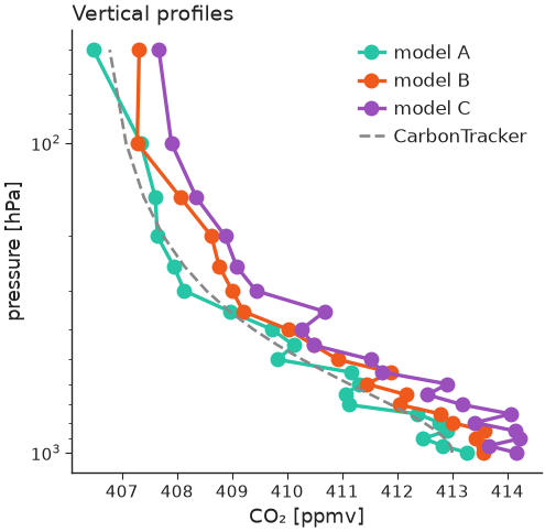
"""Vertical profiles — value vs pressure, inverted log axis, with a baseline."""

import nicefigs as nf
from nicefigs import data


def make():
    nf.set_theme("paper")
    vp = data.vertical_profiles()
    ax = nf.profile(
        vp["profiles"],
        vp["levels"],
        baselines={"CarbonTracker": vp["baseline"]},
        xlabel="CO₂",
        xunits="ppmv",
        ylabel="pressure",
        yunits="hPa",
        log_y=True,
        title="Vertical profiles",
    )
    return ax.figure


if __name__ == "__main__":
    import matplotlib

    matplotlib.use("Agg")
    nf.save(make(), "27_profile", formats=("png", "pdf"))

28 — Frame-based animation engine

nicefigs.render_animation renders each frame with your own draw(i) -> Figure callback and stitches them with nicefigs.stitch_frames (MP4 via ffmpeg, GIF fallback). A frame can be anything — here a field snapshot and a running timeseries side by side, which animate_maps alone can't do. Pass method="parallel" to fan the frames out across CPU cores for large or expensive animations.

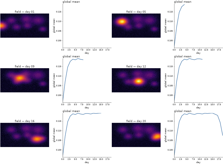
"""Frame-based animation engine — a multi-panel frame drawn per step, stitched.

``render_animation`` takes a ``draw(i) -> Figure`` callback, so a frame can be
anything (here: a map-like image *and* a running timeseries side by side —
which ``animate_maps`` alone can't do). Pass ``method="parallel"`` to render the
frames across CPU cores for large / expensive animations.
"""

import numpy as np

import nicefigs as nf
from nicefigs import data

_LON, _LAT, _FRAMES = data.map_timeseries_cube(n_frames=20, shape=(60, 120))
_GLOBAL_MEAN = _FRAMES.reshape(len(_FRAMES), -1).mean(axis=1)


def draw(i):
    """Draw frame ``i``: a field snapshot + the global-mean trace so far."""
    nf.set_theme("paper")
    fig, axes = nf.subplots(1, 2, width="full", panel_aspect=0.8, wspace=0.28)
    nf.image(
        _FRAMES[i],
        cmap="inferno",
        vmin=float(_FRAMES.min()),
        vmax=float(_FRAMES.max()),
        title=f"field — day {i + 1:02d}",
        ax=axes[0],
    )
    axes[1].plot(np.arange(i + 1), _GLOBAL_MEAN[: i + 1], color=nf.COLORS["blue"])
    axes[1].set_xlim(0, len(_FRAMES) - 1)
    axes[1].set_ylim(_GLOBAL_MEAN.min(), _GLOBAL_MEAN.max())
    nf.set_labels(axes[1], x="day", y="global mean")
    nf.clean_title(axes[1], "global mean")
    return fig


def make(path="28_render_animation.gif"):
    # method="sequential" here keeps the gallery self-contained; use
    # method="parallel" (the default) to fan frames out across cores.
    return nf.render_animation(draw, len(_FRAMES), path, fps=6, dpi=90, method="sequential")


if __name__ == "__main__":
    import matplotlib

    matplotlib.use("Agg")
    make()

29 — Timeseries with hue-mapped observations

timeseries's sparse obs= overlay can be coloured by a third variable via obs_hue (e.g. sample altitude) instead of the flat obs_color, with obs_colorbar=True drawing a slim colorbar for it. The legend still gets one proxy handle for the overlay, not one per point.

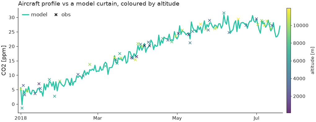
"""Timeseries — sparse observations coloured by a third variable (e.g. altitude)."""

import numpy as np

import nicefigs as nf
from nicefigs import data


def make():
    nf.set_theme("paper")
    dates, series = data.timeseries(n_days=200, series=["model"])
    rng = np.random.default_rng(0)
    idx = np.sort(rng.choice(len(dates), 60, replace=False))
    odates = [dates[i] for i in idx]
    ovals = series["model"][idx] + rng.normal(0, 1, 60)
    altitude = rng.uniform(0, 12000, 60)

    ax = nf.timeseries(
        dates,
        series,
        obs=(odates, ovals),
        obs_hue=altitude,
        obs_cmap="viridis",
        obs_hue_label="altitude [m]",
        obs_colorbar=True,
        ylabel="CO2",
        yunits="ppm",
        title="Aircraft profile vs a model curtain, coloured by altitude",
    )
    return ax.figure


if __name__ == "__main__":
    import matplotlib

    matplotlib.use("Agg")
    nf.save(make(), "29_timeseries_obs_hue", formats=("png", "pdf"))

31 — Panel label composed with an existing title

label_panels's use_ax_title=True picks up each panel's own ax.set_title() (as set by hovmoller_panels here) and redraws it next to the bold letter at one height, instead of leaving matplotlib's separately-positioned title floating at its own default spot.

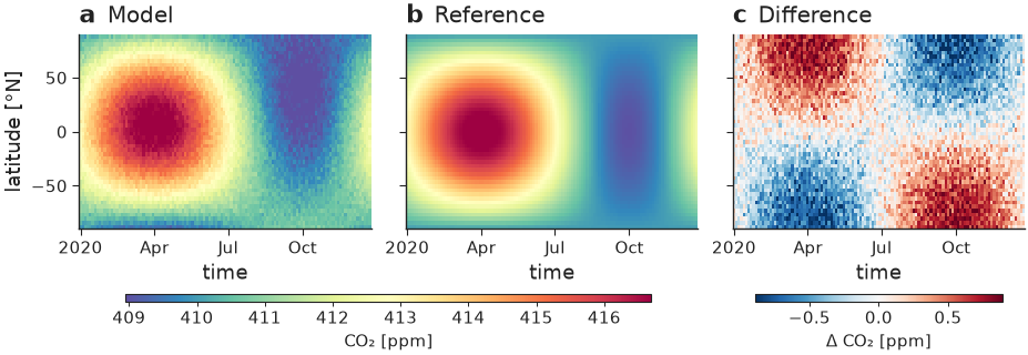
"""Panel letter + per-panel title composed onto one line.

``hovmoller_panels`` sets each panel's title via matplotlib's own
``ax.set_title`` (centred, its own default height). Calling
``label_panels(..., use_ax_title=True)`` afterwards picks that title back up,
clears it from matplotlib, and redraws it next to the bold letter at one
height — ``a  Model`` / ``b  Reference`` / ``c  Difference`` — instead of a bold
letter and a title floating at two different positions.
"""

import nicefigs as nf
from nicefigs import data


def make():
    nf.set_theme("paper")
    h = data.hovmoller_field()
    diff = h["value"] - h["reference"]
    fig, axes = nf.hovmoller_panels(
        {"Model": h["value"], "Reference": h["reference"], "Difference": diff},
        h["times"],
        h["lats"],
        diff_fields={"Difference"},
        value_label="CO₂ [ppm]",
        diff_label="Δ CO₂ [ppm]",
    )
    # Compose each panel's existing ax.set_title with the bold letter, instead
    # of letting the two render at different heights/positions.
    nf.label_panels(axes, use_ax_title=True)
    return fig


if __name__ == "__main__":
    import matplotlib

    matplotlib.use("Agg")
    nf.save(make(), "31_panel_label_with_title", formats=("png", "pdf"))